Numerical Methods Contents - SAM

−2.5 −2 −1.5 −1 −0.5 0 0.5 1 1.5 2 2.5
2.5
2
1.5
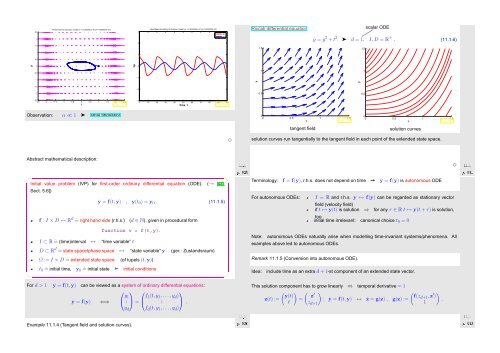
Phase flow for Zeeman model (α = 5.000000e−01,β=1.000000e−01)
3
2
Heartbeat according to Zeeman model (α = 5.000000e−01,β=1.000000e−01)
l(t)
p(t)
Riccati differential equation
1.5
ẏ = y 2 + t 2
➤
scalar ODE
d = 1, I, D = R + . (11.1.6)
1.5
1
1
0.5
p
0
l/p
0
−0.5
1
1
−1
−1
y
y
−1.5
−2
−2
0.5
0.5
−2.5
l
Fig. 128
−3
0 10 20 30 40 50 60 70 80 90 100
time t
Fig. 129
Observation: α ≪ 1 ➤ atrial fibrillation
0
0 0.5 1 1.5
t
Fig. 130
0
0 0.5 1 1.5
t
Fig. 131
tangent field
solution curves
✸
solution curves run tangentially to the tangent field in each point of the extended state space.
Abstract mathematical description:
Ôº¾ ½½º½
Ôº¿½ ½½º½ ✸
✬
Initial value problem (IVP) for first-order ordinary differential equation (ODE): (→ [40,
Sect. 5.6])
ẏ = f(t,y) , y(t 0 ) = y 0 . (11.1.5)
f : I × D ↦→ R d ˆ= right hand side (r.h.s.) (d ∈ N), given in procedural form
✩
Terminology: f = f(y), r.h.s. does not depend on time ➙ ẏ = f(y) is autonomous ODE
For autonomous ODEs:
I = R and r.h.s. y ↦→ f(y) can be regarded as stationary vector
field (velocity field)
if t ↦→ y(t) is solution ⇒ for any τ ∈ R t ↦→ y(t + τ) is solution,
too.
initial time irrelevant: canonical choice t 0 = 0
function v = f(t,y).
I ⊂ R ˆ= (time)interval ↔ “time variable” t
D ⊂ R d ˆ= state space/phase space ↔ “state variable” y (ger.: Zustandsraum)
Ω := I × D ˆ= extended state space (of tupels (t,y))
Note: autonomous ODEs naturally arise when modelling time-invariant systems/phenomena. All
examples above led to autonomous ODEs.
Remark 11.1.5 (Conversion into autonomous ODE).
✫
t 0 ˆ= initial time, y 0 ˆ= initial state ➣ initial conditions
✪
Idea:
include time as an extra d + 1-st component of an extended state vector.
For d > 1 ẏ = f(t,y) can be viewed as a system of ordinary differential equations:
⎛
ẏ = f(y) ⇐⇒ ⎝ y ⎞ ⎛
1
. ⎠ = ⎝ f ⎞
1(t,y 1 ,...,y d )
. ⎠ .
y d f d (t,y 1 , ...,y d )
Example 11.1.4 (Tangent field and solution curves).
Ôº¿¼ ½½º½
This solution component has to grow linearly ⇔ temporal derivative = 1
( ) ( )
(
y(t) z ′
f(zd+1 ,z
z(t) := = : ẏ = f(t,y) ↔ ż = g(z) , g(z) :=
′ )
)
.
t z d+1 1
Ôº¿¾ ½½º½