Numerical Methods Contents - SAM

1
∃ (partial) cyclic row permutation m + 1 ← k, i ← i + 1, i = k,...,m:
→ unitary permutation matrix (→ Def. 2.3.1) P ∈ {0, 1} m+1,m+1
( ) ( A Q
PÃ = H ( )
0 R
)PÃ v T 0 1
= v T
Fall m = n
=
⎛
⎜
⎝
v T R
⎞
⎟
⎠ .
3
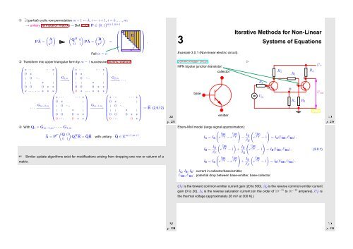
Example 3.0.1 (Non-linear electric circuit).
Iterative Methods for Non-Linear
Systems of Equations
2 Transform into upper triangular form by m − 1 successive Givens rotations:
⎛
⎞ ⎛
⎞
∗ · · · · · · ∗
∗ · · · · · · ∗
0 ∗ .
0 ∗ .
. 0 . ..
G 1,m
⎜ . . ∗ .
−−−→
. 0 ...
G 2,m
⎟ ⎜ . . ∗ .
−−−→ · · ·
⎟
⎝ 0 0 0 ∗ ∗ ⎠ ⎝ 0 0 0 ∗ ∗ ⎠
∗ · · · · · · ∗ ∗ ∗ 0 ∗ · · · ∗ ∗ ∗
⎛
⎞ ⎛
⎞
∗ · · · · · · ∗
∗ · · · · · · ∗
0 ∗ .
0 ∗ .
G m−2,m
· · · −−−−−→
. 0 . ..
G m−1,m
⎜ . . ∗ .
−−−−−→
. 0 ...
⎟ ⎜ . . ∗ .
:= ˜R (2.9.12)
⎟
⎝ 0 0 0 ∗ ∗ ⎠ ⎝ 0 0 0 ∗ ∗ ⎠
0 · · · 0 ∗ ∗
0 · · · 0 ∗
Ôº¾¿¿ ¾º
Schmitt trigger circuit
NPN bipolar junction transistor:
collector
base
emitter
✄
R b
U in
➄
➀
U +
R 3 R 4
R 1
➃
➂
➁
U out
R e R 2
Fig. 27
Ôº¾¿ ¿º¼
3 With Q 1 = G m−1,m · · · · · G 1,m
( )
à = P T Q 0
Q
0 1
H 1 ˜R = ˜Q˜R with unitary ˜Q ∈ K m+1,m+1 .
☞
matrix.
Similar update algorithms exist for modifications arising from dropping one row or column of a
Ebers-Moll model (large signal approximation):
) ( )
U BE U BC
I C = I S
(e
U T − e
U T − I U BC
S
e
U T − 1 = I
β C (U BE , U BC ) ,
R
I B = I (
U
) ( )
BE
S
e
U T − 1 + I U BC
S
e
U T − 1 = I B (U BE , U
β F β BC ) ,
R
)
U BE U BC
I E = I S
(e
U T − e
U T + I (
S
β F
)
U T − 1 = I E (U BE ,U BC ) .
U BE
e
I C , I B , I E : current in collector/base/emitter,
U BE , U BC : potential drop between base-emitter, base-collector.
(3.0.1)
(β F is the forward common emitter current gain (20 to 500), β R is the reverse common emitter current
gain (0 to 20), I S is the reverse saturation current (on the order of 10 −15 to 10 −12 amperes), U T is
the thermal voltage (approximately 26 mV at 300 K).)
Ôº¾¿ ¾º
Ôº¾¿ ¿º¼