Numerical Methods Contents - SAM

approximation of Φ:
Φ(x) ≈ Q(s) := Φ(x (k) ) + grad Φ(x (k) ) T s + 1 2 sT HΦ(x (k) )s , (6.5.6)
grad Q(s) = 0 ⇔ HΦ(x (k) )s + grad Φ(x (k) ) = 0 ⇔ (6.5.5) .
➣ Another model function method (→ Sect. 3.3.2) with quadratic model function for Q.
△
MATLAB-\ used to solve linear least squares problem
in each step:
for A ∈ R m,n
x = A\b
↕
x minimizer of ‖Ax − b‖ 2
with minimal 2-norm
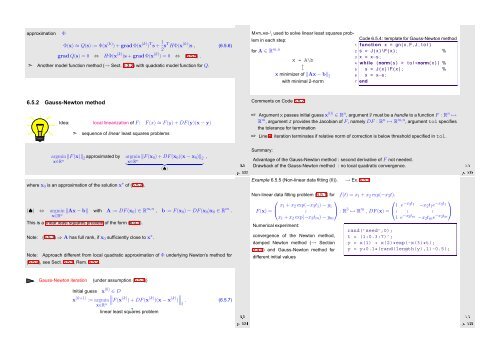
Code 6.5.4: template for Gauss-Newton method
1 function x = gn ( x , F , J , t o l )
2 s = J ( x ) \ F ( x ) ; %
3 x = x−s ;
4 while (norm( s ) > t o l ∗norm( x ) ) %
5 s = J ( x ) \ F ( x ) ; %
6 x = x−s ;
7 end
6.5.2 Gauss-Newton method
Idea: local linearization of F : F(x) ≈ F(y) + DF(y)(x − y)
➣ sequence of linear least squares problems
Comments on Code 6.5.2:
☞ Argument x passes initial guess x (0) ∈ R n , argument F must be a handle to a function F : R n ↦→
R m , argument J provides the Jacobian of F , namely DF : R n ↦→ R m,n , argument tol specifies
the tolerance for termination
☞ Line 4: iteration terminates if relative norm of correction is below threshold specified in tol.
argmin ‖F(x)‖
x∈R n 2 approximated by argmin
‖F(x 0) + DF(x 0 )(x − x 0 )‖ 2 ,
} x∈R n {{ }
(♠)
Ôº¿¿ º
Summary:
Advantage of the Gauss-Newton method : second derivative of F not needed.
Drawback of the Gauss-Newton method : no local quadratic convergence.
Ôº¿ º
where x 0 is an approximation of the solution x ∗ of (6.5.2).
(♠) ⇔
argmin
x∈R n ‖Ax − b‖ with A := DF(x 0 ) ∈ R m,n , b := F(x 0 ) − DF(x 0 )x 0 ∈ R m .
This is a linear least squares problem of the form (6.0.3).
Note: (6.5.3) ⇒ A has full rank, if x 0 sufficiently close to x ∗ .
Note:
Approach different from local quadratic approximation of Φ underlying Newton’s method for
(6.5.2), see Sect. 6.5.1, Rem. 6.5.2.
Example 6.5.5 (Non-linear data fitting (II)). → Ex. 6.5.1
Non-linear data fitting problem (6.5.1) for f(t) = x 1 + x 2 exp(−x 3 t).
⎛
F(x) = ⎝ x ⎞
⎛
1 + x 2 exp(−x 3 t 1 ) − y 1
. ⎠ : R 3 ↦→ R m , DF(x) = ⎝ 1 e−x 3t 1 −x2 t 1 e −x ⎞
3t 1
. .
. ⎠
x 1 + x 2 exp(−x 3 t m ) − y m 1 e −x 3t m −x2 t m e −x 3t m
Numerical experiment:
convergence of the Newton method,
damped Newton method (→ Section
3.4.4) and Gauss-Newton method for
different initial values
rand(’seed’,0);
t = (1:0.3:7)’;
y = x(1) + x(2)*exp(-x(3)*t);
y = y+0.1*(rand(length(y),1)-0.5);
Gauss-Newton iteration (under assumption (6.5.3))
Initial guess x (0) ∈ D
∥ x (k+1) ∥∥F(x
:= argmin
(k) ) + DF(x (k) )(x − x (k) ) ∥ . (6.5.7)
x∈R n 2
linear least squares problem
Ôº¿ º
Ôº¿ º