Numerical Methods Contents - SAM

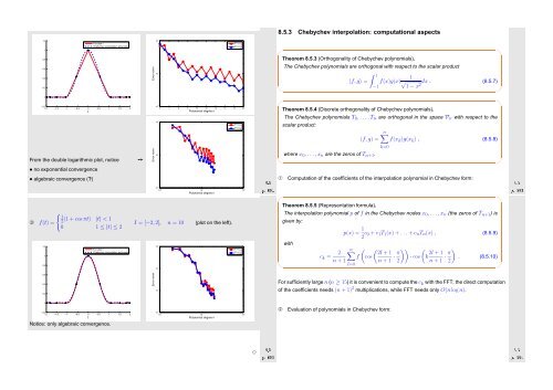
8.5.3 Chebychev interpolation: computational aspects
1.2
1
Function f
Chebychev interpolation polynomial
||f−p n
|| ∞
||f−p n
|| 2
✬
✩
0.8
Theorem 8.5.3 (Orthogonality of Chebychev polynomials).
0.6
0.4
0.2
Error norm
10 −1
The Chebychev polynomials are orthogonal with respect to the scalar product
∫ 1 1
〈f,g〉 = f(x)g(x) √ dx . (8.5.7)
−1 1 − x 2
✫
✪
0
✬
✩
−0.2
−2 −1.5 −1 −0.5 0 0.5 1 1.5 2
t
From the double logarithmic plot, notice
• no exponential convergence
• algebraic convergence (?)
➙
Error norm
10 0 Polynomial degree n
10 −2
2 4 6 8 10 12 14 16 18 20
||f−p n
|| ∞
||f−p n
|| 2
10 −1
10 −2
10 0 10 1 10 2
10 0 Polynomial degree n
Ôº½ º
Theorem 8.5.4 (Discrete orthogonality of Chebychev polynomials).
The Chebychev polynomials T 0 , ...,T n are orthogonal in the space P n with respect to the
scalar product:
n∑
(f, g) = f(x k )g(x k ) , (8.5.8)
k=0
where x 0 , ...,x n are the zeros of T n+1 .
✫
✪
Ôº¿ º
➀ Computation of the coefficients of the interpolation polynomial in Chebychev form:
✬
✩
➂ f(t) =
{ 12 (1 + cos πt) |t| < 1
0 1 ≤ |t| ≤ 2
I = [−2, 2], n = 10 (plot on the left).
Theorem 8.5.5 (Representation formula).
The interpolation polynomial p of f in the Chebychev nodes x 0 , ...,x n (the zeros of T n+1 ) is
given by:
p(x) = 1 2 c 0 + c 1 T 1 (x) + ... + c n T n (x) , (8.5.9)
1.2
1
0.8
Function f
Chebychev interpolation polynomial
10 −1
||f−p n
|| ∞
||f−p n
|| 2
with
✫
c k = 2
n + 1
n∑
l=0
( ( 2l + 1
f cos
n + 1 · π )) (
· cos k 2l + 1
2 n + 1 · π )
. (8.5.10)
2
✪
0.6
0.4
0.2
Error norm
10 −2
For sufficiently large n (n ≥ 15) it is convenient to compute the c k with the FFT; the direct computation
of the coefficients needs (n + 1) 2 multiplications, while FFT needs only O(n log n).
0
−0.2
−2 −1.5 −1 −0.5 0 0.5 1 1.5 2
t
Notice: only algebraic convergence.
10 0 Polynomial degree n
10 −3
10 0 10 1 10 2
➁
Evaluation of polynomials in Chebychev form:
Ôº¾ º
✸
Ôº º