Numerical Methods Contents - SAM

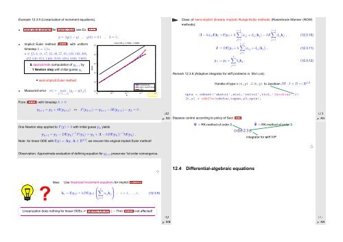
Example 12.3.5 (Linearization of increment equations).
Initial value problem for logistic ODE, see Ex. 11.1.1
Implicit Euler method (11.2.4) with uniform
timestep h = 1/n,
n ∈ {5, 8, 11, 17, 25, 38, 57, 85, 128, 192, 288,
, 432, 649, 973, 1460, 2189, 3284, 4926, 7389}.
& approximate computation of y k+1 by
1 Newton step with initial guess y k
ẏ = λy(1 − y) , y(0) = 0.1 , λ = 5 .
error
10 −1
10 −2
10 −3
Logistic ODE, y 0
= 0.100000, λ = 5.000000
Class of semi-implicit (linearly implicit) Runge-Kutta methods (Rosenbrock-Wanner (ROW)
methods):
∑i−1
∑i−1
(I − ha ii J)k i =f(y 0 + h (a ij + d ij )k j ) − hJ d ij k j , (12.3.10)
j=1
j=1
J := Df ( ∑i−1
)
y 0 + h (a ij + d ij )k j , (12.3.11)
y 1 :=y 0 +
j=1
s∑
b j k j . (12.3.12)
j=1
Remark 12.3.6 (Adaptive integrator for stiff problems in MATLAB).
10 0 h
= semi-implicit Euler method
Measured error err = max
j=1,...,n |y j − y(t j )|
From (11.2.4) with timestep h > 0
10 −4
implicit Euler
semi−implicit Euler
O(h)
10 −5
10 −4 10 −3 10 −2 10 −1 10 0
Fig. 170
y k+1 = y k + hf(y k+1 ) ⇔ F(y k+1 ) := y k+1 − hf(y k+1 ) − y k
Ôº¿¿ ½¾º¿
= 0 .
Handle of type @(t,y) J(t,y) to Jacobian Df : I × D ↦→ R d,d
opts = odeset(’abstol’,atol,’reltol’,rtol,’Jacobian’,J)
[t,y] = ode23s(odefun,tspan,y0,opts);
Stepsize control according to policy of Sect. 11.5:
Ôº¿ ½¾º¿
One Newton step applied to F(y) = 0 with initial guess y k yields
y k+1 = y k − Df(y k ) −1 F(y k ) = y k + (I − hDf(y k )) −1 hf(y k ) .
Note: for linear ODE with f(y) = Ay, A ∈ R d,d , we recover the original implicit Euler method!
Observation: Approximate evaluation of defining equation for y k+1 preserves 1st order convergence.
Ψ ˆ= RK-method of order 2 ˜Ψ ˆ= RK-method of order 3
ode23s
integrator for stiff IVP
△
✸
12.4 Differential-algebraic equations
✗
✖
?Idea:
Use linearized increment equations for implicit RK-SSM
⎛ ⎞
s∑
k i = f(y 0 ) + hDf(y 0 ) ⎝ a ij k j
⎠ , i = 1,...,s . (12.3.9)
Linearization does nothing for linear ODEs ➢ stability function (→ Thm. 12.3.2) not affected!
j=1
✔
✕
Ôº¿ ½¾º¿
Ôº¿ ½¾º