Numerical Methods Contents - SAM

Notice: rank(A) = n ⇒ A H A ∈ R n,n s.p.d. (→ Def. 2.7.1)
A way to avoid the computation of A H A:
Remark 6.1.1 (Conditioning of normal equations).
!
Caution: danger of instability, with SVD A = UΣV H
cond 2 (A H A) = cond 2 (VΣ H U H UΣV H ) = cond 2 (Σ H Σ) = σ2 1
σn
2 = cond 2 (A) 2 .
➣ For fairly ill-conditioned A using the normal equations (6.1.2) to solve the linear least squares
problem (6.1.1) numerically may run the risk of huge amplification of roundoff errors incurred
during the computation of the right hand side A H b: potential instability (→ Def. 2.5.5) of normal
equation approach.
△
Expand normal equations (6.1.2): introduce residual r := Ax − b as new unknown:
( ( )( ) (
A H Ax = A H r −I A r b
b ⇔ B :=
x)
A H = . (6.1.3)
0 x 0)
More general substitution r := α −1 (Ax − b), α > 0 to improve the condition:
( ) ( ) ( ) (
A H Ax = A H r −αI A r b
b ⇔ B α :=
x A H = . (6.1.4)
0 x 0)
For m, n ≫ 1, A sparse, both (6.1.3) and (6.1.4) lead to large sparse linear systems of equations,
amenable to sparse direct elimination techniques, see Sect. 2.6.3
Example 6.1.2 (Instability of normal equations).
Ôº¼ º½
Ôº½½ º½
!
If δ < √ eps ⇒
Caution: loss of information in the computation
of A H A, e.g.
⎛
A = ⎝ 1 1
⎞
( )
δ 0⎠ ⇒ A H 1 + δ 2 1
A =
0 δ
1 1 + δ 2
Sect. 2.4, in particular Rem. 2.4.9.
1 >> A = [1 1 ; . . .
2 sqrt ( eps ) 0 ; . . .
3 0 sqrt ( eps ) ] ;
4 >> rank (A)
5 ans = 2
6 >> rank (A’∗A)
7 ans = 1
1 + δ 2 = 1 in M, i.e. A H A “numeric singular”, though rank(A) = 2, see
✸
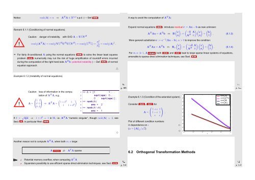
Example 6.1.3 (Condition of the extended system).
Consider (6.1.3), (6.1.4) for
⎛
A = ⎝ 1 + ǫ 1
⎞
1 − ǫ 1 ⎠ .
ǫ ǫ
Plot of different condition numbers
in dependence on ǫ
✄
(α = ‖A‖ 2 / √ 2)
10 9
10 8
10 7
10 6
10 5
10 4
10 3
10 2
10 1
✸
10 0
−5 10
cond 2
(A)
cond 2
(A H A)
cond 2
(B)
cond 2
(B α
)
10 −4 10 −3 10 −2 10 −1 10 0
10 10 ε
Another reason not to compute A H A, when both m, n large:
A sparse ⇏ A T A sparse
Potential memory overflow, when computing A T A
Squanders possibility to use efficient sparse direct elimination techniques, see Sect. 2.6.3
Ôº½¼ º½
6.2 Orthogonal Transformation Methods
Ôº½¾ º¾