

Numerical Methods Contents - SAM
Numerical Methods Contents - SAM
Numerical Methods Contents - SAM

You also want an ePaper? Increase the reach of your titles
YUMPU automatically turns print PDFs into web optimized ePapers that Google loves.
5.5 Singular Value Decomposition<br />
Remark 5.5.1 (Principal component analysis (PCA)).<br />
Given: n data points a j ∈ R m , j = 1, ...,n, in m-dimensional (feature) space<br />
⎛<br />
⎜<br />
⎝<br />
A<br />
⎞ ⎛<br />
⎟<br />
⎠ = ⎜<br />
⎝<br />
U<br />
⎞ ⎛<br />
⎟ ⎜<br />
⎠ ⎝<br />
Σ<br />
⎛<br />
⎞<br />
⎟<br />
⎠<br />
⎜<br />
⎝<br />
V H<br />
⎞<br />
⎟<br />
⎠<br />
Conjectured: “linear dependence”: a j ∈ V , V ⊂ R m p-dimensional subspace,<br />
p < min{m, n} unknown<br />
(➣ possibility of dimensional reduction)<br />
Task (PCA):<br />
Perspective of linear algebra:<br />
Extension:<br />
determine (minimal) p and (orthonormal basis of) V<br />
Conjecture ⇔ rank(A) = p for A := (a 1 , ...,a n ) ∈ R m,n , Im(A) = V<br />
Data affected by measurement errors<br />
(but conjecture upheld for unperturbed data)<br />
△<br />
Ôº½ º<br />
Proof. (of Thm. 5.5.1, by induction)<br />
[40, Thm. 4.2.3]: Continuous functions attain extremal values on compact sets (here the unit ball<br />
{x ∈ R n : ‖x‖ 2 ≤ 1})<br />
➤ ∃x ∈ K n ,y ∈ K m , ‖x‖ = ‖y‖ 2 = 1 : Ax = σy , σ = ‖A‖ 2 ,<br />
where we used the definition of the matrix 2-norm, see Def. 2.5.2. By<br />
Gram-Schmidt orthogonalization: ∃Ṽ ∈ Kn,n−1 , Ũ ∈ Km,m−1 such that<br />
V = (x Ṽ) ∈ Kn,n , U = (y Ũ) ∈ Km,m are unitary.<br />
(<br />
)<br />
U H AV = (y Ũ)H A(x Ṽ) = y H Ax y H AṼ<br />
Ũ H Ax ŨH AṼ<br />
(<br />
σ w<br />
Ôº¿ º<br />
)<br />
H<br />
= =: A<br />
0 B 1 .<br />
✬<br />
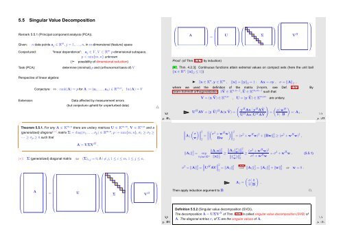
Theorem 5.5.1. For any A ∈ K m,n there are unitary matrices U ∈ K m,m , V ∈ K n,n and a<br />
(generalized) diagonal (∗) matrix Σ = diag(σ 1 , ...,σ p ) ∈ R m,n , p := min{m, n}, σ 1 ≥ σ 2 ≥<br />
· · · ≥ σ p ≥ 0 such that<br />
✫<br />
A = UΣV H .<br />
(∗): Σ (generalized) diagonal matrix :⇔ (Σ) i,j = 0, if i ≠ j, 1 ≤ i ≤ m, 1 ≤ j ≤ n.<br />
⎛<br />
⎜<br />
⎝<br />
A<br />
⎞<br />
⎛<br />
=<br />
⎟ ⎜<br />
⎠ ⎝<br />
U<br />
⎞⎛<br />
⎟<br />
⎠⎜<br />
⎝<br />
Σ<br />
⎞<br />
⎛<br />
⎜<br />
⎝<br />
⎟<br />
⎠<br />
V H<br />
⎞<br />
⎟<br />
⎠<br />
✩<br />
✪<br />
Ôº¾ º<br />
Since<br />
( )∥ σ ∥∥∥ 2<br />
(<br />
∥ A 1 =<br />
σ 2 + w H )∥<br />
w ∥∥∥ 2<br />
w ∥<br />
= (σ 2 + w H w) 2 + ‖Bw‖ 2<br />
2 Bw<br />
2 ≥ (σ2 + w H w) 2 ,<br />
2<br />
we conclude<br />
‖A 1 ‖ 2 2 = sup ‖A 1 x‖ 2 ∥ (<br />
2<br />
∥A σw )∥<br />
1<br />
∥ 2<br />
0≠x∈K n ‖x‖ 2 ≥ 2<br />
∥ ( σ)∥ ≥ (σ2 + w H w) 2<br />
2 ∥ 2 σ 2 + w H w = σ2 + w H w . (5.5.1)<br />
w 2<br />
∥ σ 2 = ‖A‖ 2 ∥∥U<br />
2 = H AV∥ 2 = ‖A 1‖ 2<br />
2<br />
2<br />
(5.5.1)<br />
=⇒ ‖A 1 ‖ 2 2 = ‖A 1‖ 2 2 + ‖w‖2 2 ⇒ w = 0 .<br />
( )<br />
σ 0<br />
A 1 = .<br />
0 B<br />
Then apply induction argument to B ✷.<br />
Ôº º<br />
A. The diagonal entries σ i of Σ are the singular values of A.<br />
Definition 5.5.2 (Singular value decomposition (SVD)).<br />
The decomposition A = UΣV H of Thm. 5.5.1 is called singular value decomposition (SVD) of


