Numerical Methods Contents - SAM

1
0.9
Function f
1
0.9
Function f
✬
Lemma 9.5.3 (Properties of Bernstein polynomials).
✩
0.8
0.8
(i) t = 0 is a zero of order i of b i,n , t = 1 is a zero of order n − i of b i,n ,
0.7
0.6
0.5
0.7
0.6
0.5
(ii)
(iii)
∑ n
i=0 b i,n ≡ 1 (partition of unity),
b i,n (t) = (1 − t) b i,n−1 + t b i−1,n−1 (t),
0.4
0.4
(iv) b i,n (t) ≥ 0 ∀ 0 ≤ t ≤ 1.
0.3
0.3
✫
✪
0.2
0.2
0.1
0
0 0.2 0.4 0.6 0.8 1
t
0.1
0
0 0.2 0.4 0.6 0.8 1
t
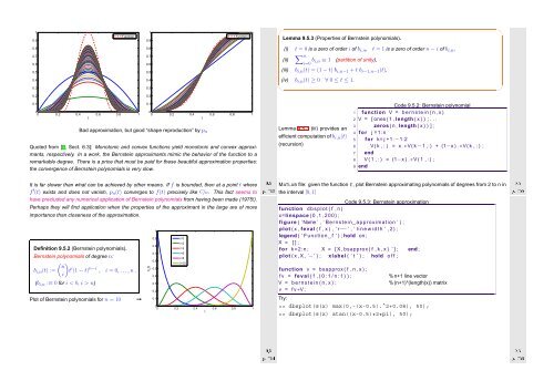
Bad approximation, but good “shape reproduction” by p n
Quoted from [9, Sect. 6.3]: Monotonic and convex functions yield monotonic and convex approximants,
respectively. In a work, the Bernstein approximants mimic the behavior of the function to a
remarkable degree. There is a price that must be paid for these beautiful approximation properties:
the convergence of Bernstein polynomials is very slow.
Ôº¿ º
f ′ (t) exists and does not vanish, p n (t) converges to f(t) precisely like C/n. This fact seems to
It is far slower than what can be achieved by other means. If f is bounded, then at a point t where
have precluded any numerical application of Bernstein polynomials from having been made (1975!).
Perhaps they will find application when the properties of the approximant in the large are of more
importance than closeness of the approximation.
Definition 9.5.2 (Bernstein polynomials).
Bernstein polynomials of degree n:
( n
b i,n (t) := t
i)
i (1 − t) n−i , i = 0, ...,n .
(b i,n :≡ 0 for i < 0, i > n)
Plot of Bernstein polynomials for n = 10
➙
b n
(t)
1
0.9
0.8
0.7
0.6
0.5
0.4
0.3
0.2
0.1
i=0
i=2
i=4
i=6
i=8
i=10
0
0 0.2 0.4 0.6 0.8 1
t
Lemma 9.5.3 (iii) provides an
efficient computation of b i,n (t)
(recursion)
Code 9.5.2: Bernstein polynomial
1 function V = b e r n s t e i n ( n , x )
2 V = [ ones ( 1 , length ( x ) ) ; . . .
3 zeros ( n , length ( x ) ) ] ;
4 for j =1:n
5 for k= j +1:−1:2
6 V( k , : ) = x .∗V( k −1 ,:) + (1−x ) .∗V( k , : ) ;
7 end
8 V ( 1 , : ) = (1−x ) .∗V ( 1 , : ) ;
9 end
MATLAB file: given the function f, plot Bernstein approximating polynomials of degrees from 2 to n in
the interval [0, 1]
1 function d b splot ( f , n )
2 x=linspace (0 ,1 ,200) ;
Code 9.5.3: Bernstein approximation
3 figure ( ’Name ’ , ’ Bernstein approximation ’ ) ;
4 plot ( x , feval ( f , x ) , ’ r−−’ , ’ l i n e w i d t h ’ ,2) ;
5 legend ( ’ Function f ’ ) ; hold on ;
6 X = [ ] ;
7 for k =2:n ; X = [ X, bsapprox ( f , k , x ) ’ ] ; end ;
8 plot ( x , X, ’− ’ ) ; xlabel ( ’ t ’ ) ; hold o f f ;
9
10 function v = bsapprox ( f , n , x ) ;
11 f v = feval ( f , ( 0 : 1 / n : 1 ) ) ; % n+1 line vector
12 V = b e r n s t e i n ( n , x ) ; % (n+1)*(length(x)) matrix
13 v = f v ∗V ;
Try:
>> dbsplot(@(x) max(0,-(x-0.5).^2+0.08), 50);
>> dbsplot(@(x) atan((x-0.5)*2*pi), 50);
Ôº º
Ôº º
Ôº º