Numerical Methods Contents - SAM

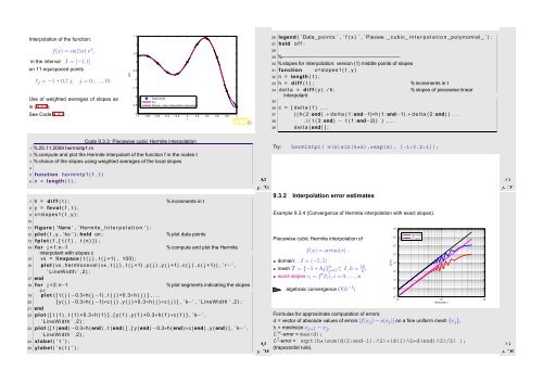
Interpolation of the function:
f(x) = sin(5x) e x ,
in the interval I = [−1, 1]
on 11 equispaced points
t j = −1 + 0.2 j, j = 0,...,10.
Use of weighted averages of slopes as
in (9.3.3).
s(t)
−0.5
−1.5
−2.5
See Code 9.3.2.
−3
−1 −0.8 −0.6 −0.4 −0.2 0 0.2 0.4 0.6 0.8 1
1.5
1
0.5
0
−1
−2
Data points
f(x)
Piecew. cubic interpolation polynomial
t
Fig. 106 ✸
26 legend ( ’ Data p o i n t s ’ , ’ f ( x ) ’ , ’ Piecew . cubic i n t e r p o l a t i o n polynomial ’ ) ;
27 hold o f f ;
28
29 %———————————————————————–
30 % slopes for interpolation: version (1) middle points of slopes
31 function c=slopes1 ( t , y )
32 n = length ( t ) ;
33 h = d i f f ( t ) ; % increments in t
34 d e l t a = d i f f ( y ) . / h ; % slopes of piecewise linear
interpolant
35
36 c = [ d e l t a ( 1 ) , . . .
37 ( ( h ( 2 : end ) .∗ d e l t a ( 1 : end−1)+h ( 1 : end−1) .∗ d e l t a ( 2 : end ) ) . . .
38 . / ( t ( 3 : end ) − t ( 1 : end−2) ) ) , . . .
39 d e l t a ( end ) ] ;
Code 9.3.3: Piecewise cubic Hermite interpolation
1 % 25.11.2009 hermintp1.m
2 % compute and plot the Hermite interpolant of the function f in the nodes t
3 % choice of the slopes using weighted averages of the local slopes
Ôº¼ º¿
6 n = length ( t ) ;
4
5 function hermintp1 ( f , t )
7 h = d i f f ( t ) ; % increments in t
8 y = feval ( f , t ) ;
9 c=slopes1 ( t , y ) ;
10
Try: hermintp1( @(x)sin(5*x).*exp(x), [-1:0.2:1]);
9.3.2 Interpolation error estimates
Example 9.3.4 (Convergence of Hermite interpolation with exact slopes).
Ôº¼ º¿
11 figure ( ’Name ’ , ’ Hermite I n t e r p o l a t i o n ’ ) ;
12 plot ( t , y , ’ ko ’ ) ; hold on ; % plot data points
13 f p l o t ( f , [ t ( 1 ) , t ( n ) ] ) ;
14 for j =1:n−1 % compute and plot the Hermite
interpolant with slopes c
15 vx = linspace ( t ( j ) , t ( j +1) , 100) ;
16 plot ( vx , hermloceval ( vx , t ( j ) , t ( j +1) , y ( j ) , y ( j +1) , c ( j ) , c ( j +1) ) , ’ r−’ ,
’ LineWidth ’ ,2) ;
17 end
18 for j =2:n−1 % plot segments indicating the slopes
c-i
19 plot ( [ t ( j ) −0.3∗h ( j −1) , t ( j ) +0.3∗h ( j ) ] , . . .
20 [ y ( j ) −0.3∗h ( j −1)∗c ( j ) , y ( j ) +0.3∗h ( j ) ∗c ( j ) ] , ’ k−’ , ’ LineWidth ’ ,2) ;
21 end
22 plot ( [ t ( 1 ) , t ( 1 ) +0.3∗h ( 1 ) ] , [ y ( 1 ) , y ( 1 ) +0.3∗h ( 1 ) ∗c ( 1 ) ] , ’ k−’ ,
’ LineWidth ’ ,2) ;
23 plot ( [ t ( end ) −0.3∗h ( end ) , t ( end ) ] , [ y ( end ) −0.3∗h ( end ) ∗c ( end ) , y ( end ) ] , ’ k−’ ,
Ôº¼ º¿
’ LineWidth ’ ,2) ;
24 xlabel ( ’ t ’ ) ;
25 ylabel ( ’ s ( t ) ’ ) ;
Piecewise cubic Hermite interpolation of
f(x) = arctan(x) .
domain: I = (−5, 5)
mesh T = {−5 + hj} n j=0 ⊂ I, h = 10
n ,
exact slopes c i = f ′ (t i ), i = 0,...,n
algebraic convergence O(h −4 )
||s−f||
sup−norm
L 2 −norm
10 2
10 1
10 0
10 −1
10 −2
10 −3
10 −4
10 −5
10 −6
10 −1 10 0
Meshwidth h
10 1
Formulas for approximate computation of errors:
d = vector of absolute values of errors |f(x j ) − s(x j )| on a fine uniform mesh {x j },
h = meshsize x j+1 − x j ,
L ∞ -error = max(d);
L 2 -error = sqrt(h*(sum(d(2:end-1).∧2)+(d(1)∧2+d(end)∧2)/2) );
(trapezoidal rule).
Ôº¼ º¿