Numerical Methods Contents - SAM

Initial guess x (0) ∈ R n , k = 0
r 0 := b − Ax (0)
repeat
t ∗ := rT k r k
r T k Ar k
x (k+1) := x (k) + t ∗ r k
r k+1 := r k − t ∗ Ar k
k := k + 1
∥
until ∥x (k) − x (k−1)∥ ∥
∥ ∥ ∥∥x ≤τ (k) ∥
Code 4.1.6: gradient method for Ax = b, A s.p.d.
1 function x = g r a d i t (A, b , x , t o l , maxit )
2 r = b−A∗x ;
3 for k =1: maxit
4 p = A∗ r ;
5 t s = ( r ’∗ r ) / ( r ’∗ p ) ;
6 x = x + t s ∗ r ;
7 i f ( abs ( t s ) ∗norm( r ) < t o l ∗norm( x ) )
8 return ; end
9 r = r − t s ∗p ;
10 end
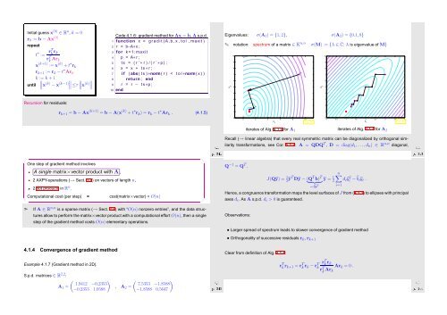
Eigenvalues: σ(A 1 ) = {1, 2}, σ(A 2 ) = {0.1, 8}
✎ notation: spectrum of a matrix ∈ K n,n σ(M) := {λ ∈ C: λ is eigenvalue of M}
x 2
10
9
8
x (0)
7
6
5
4
x 2
10
9
8
7
6
5
4
x (1) x (2)
Recursion for residuals:
r k+1 = b − Ax (k+1) = b − A(x (k) + t ∗ r k ) = r k − t ∗ Ar k . (4.1.5)
3
2
1
3
2
1
x (3) x 1
Ôº¿½ º½
0
0 2 4 6 8 10
0
0 0.5 1 1.5 2 2.5 3 3.5 4
Fig. 44
x 1
iterates of Alg. 4.1.4 for A 1 iterates of Alg. 4.1.4 for A 2
Recall (→ linear algebra) that every real symmetric matrix can be diagonalized by orthogonal similarity
transformations, see Cor. 5.1.7: A = QDQ T , D = diag(d 1 ,...,d n ) ∈ R n,n diagonal,
Fig. 45
Ôº¿¿ º½
✬
One step of gradient method involves
A single matrix×vector product with A ,
2 AXPY-operations (→ Sect. 1.4) on vectors of length n,
2 dot products in R n .
Computational cost (per step) = cost(matrix×vector) + O(n)
✫
✩
✪
Q −1 = Q T .
J(Qŷ) = 1 2ŷT Dŷ − (Q T b) T
} {{ }
=:̂b T ŷ = 1 2
n∑
d i ŷi 2 −̂b i ŷ i .
Hence, a congruence transformation maps the level surfaces of J from (4.1.1) to ellipses with principal
axes d i . As A s.p.d. d i > 0 is guaranteed.
i=1
➣
If A ∈ R n,n is a sparse matrix (→ Sect. 2.6) with “O(n) nonzero entries”, and the data structures
allow to perform the matrix×vector product with a computational effort O(n), then a single
step of the gradient method costs O(n) elementary operations.
Observations:
• Larger spread of spectrum leads to slower convergence of gradient method
• Orthogonality of successive residuals r k , r k+1
4.1.4 Convergence of gradient method
Clear from definition of Alg. 4.1.4:
Example 4.1.7 (Gradient method in 2D).
S.p.d. matrices ∈ R 2,2 :
A 1 =
( )
1.9412 −0.2353
−0.2353 1.0588
, A 2 =
Ôº¿¾ º½
( )
7.5353 −1.8588
−1.8588 0.5647
r T k r k+1 = r T k r k − r T r T k r k
k
r T k Ar Ar k = 0 .
k
Ôº¿ º½