Numerical Methods Contents - SAM

For fixed local n-point quadrature rule: O(mn) f-evaluations for composite quadrature (“total cost”)
➣ If mesh equidistant (|x j −x j−1 | = h for all j), then total cost for composite numerical quadrature
= O(h −1 ).
✬
Theorem 10.3.1 (Convergence of composite quadrature formulas).
For a composite quadrature formula Q based on a local quadrature formula of order p ∈ N
holds
✫
∃C > 0:
∫
∥ ∣ f(t) dt − Q(f) ∣ ≤ Ch p ∥ ∥f
(p) ∥L
I
∞ (I)
Proof. Apply interpolation error estimate (9.2.1).
∀f ∈ C p (I), ∀M .
✩
✪
✷
7 res = [ ] ;
8 for n = N
9 h = ( b−a ) / n ;
10 x = ( a : h / 2 : b ) ;
11 f v = feval ( f n c t , x ) ;
12 v a l = sum( h∗( f v ( 1 : 2 : end−2)+4∗ f v ( 2 : 2 : end−1)+ f v ( 3 : 2 : end ) ) ) / 6 ;
13 res = [ res ; h , v a l ] ;
14 end
Note: fnct is supposed to accept vector arguments and return the function value for each vector
component!
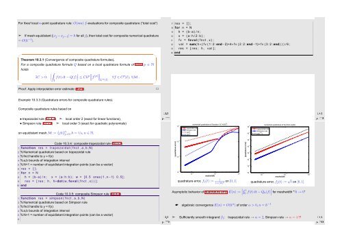
Example 10.3.3 (Quadrature errors for composite quadrature rules).
Ôº ½¼º¿
Composite quadrature rules based on
• trapezoidal rule (11.4.2) ➣ local order 2 (exact for linear functions),
• Simpson rule (10.2.4) ➣ local order 3 (exact for quadratic polynomials)
on equidistant mesh M := {jh} n j=0 , h = 1/n, n ∈ N.
numerical quadrature of function 1/(1+(5t) 2 )
10 0 trapezoidal rule
Simpson rule
O(h 2 )
O(h 4 )
numerical quadrature of function sqrt(t)
10 0 trapezoidal rule
Simpson rule
10 −1 O(h 1.5 )
Ôº ½¼º¿
Code 10.3.4: composite trapezoidal rule (10.3.2)
1 function res = t r a p e z o i d a l ( f n c t , a , b ,N)
2 % Numerical quadrature based on trapezoidal rule
3 % fnct handle to y = f(x)
4 % a,b bounds of integration interval
5 % N+1 = number of equidistant integration points (can be a vector)
6 res = [ ] ;
7 for n = N
8 h = ( b−a ) / n ; x = ( a : h : b ) ; w = [ 0 . 5 ones ( 1 , n−1) 0 . 5 ] ;
9 res = [ res ; h , h∗dot (w, feval ( f n c t , x ) ) ] ;
10 end
Code 10.3.5: composite Simpson rule (10.3.3)
1 function res = simpson ( f n c t , a , b ,N)
2 % Numerical quadrature based on Simpson rule
3 % fnct handle to y = f(x)
4 % a,b bounds of integration interval
5 % N+1 = number of equidistant integration points (can be a vector)
6
Ôº ½¼º¿
|quadrature error|
10 −5
10 −10
10 −15
10 −2 10 −1 10 0
meshwidth
2 on [0, 1] quadrature error, f 1 (t) := 1
1+(5t) quadrature error, f 2 (t) := √ t on [0, 1]
10 −2 10 −1 10 0
meshwidth
Asymptotic behavior of quadrature error E(n) := ∣ ∫ 1
0 f(t) dt − Q n (f) ∣ for meshwidth "‘h → 0”
☛
algebraic convergence E(n) = O(h α ) of order α > 0, n = h −1
|quadrature error|
10 −2
10 −3
10 −4
10 −5
10 −6
10 −7
Ôº¼ ½¼º¿
➣ Sufficiently smooth integrand f 1 : trapezoidal rule → α = 2, Simpson rule → α = 4 !?