Numerical Methods Contents - SAM

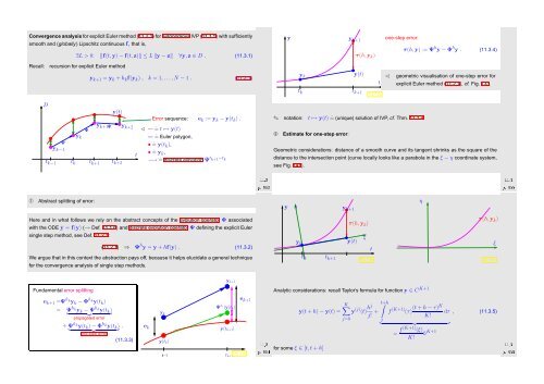
Convergence analysis for explicit Euler method (11.2.1) for autonomous IVP (11.1.5) with sufficiently
smooth and (globally) Lipschitz continuous f, that is,
∃L > 0: ‖f(t,y) − f(t,z)‖ ≤ L ‖y − z‖ ∀y,z ∈ D . (11.3.1)
Recall: recursion for explicit Euler method
y k+1 = y k + h k f(y k ) , k = 1, ...,N − 1 . (11.2.1)
y
y k+1
τ(h,y k )
y k y(t)
t
one-step error:
τ(h,y) := Ψ h y − Φ h y . (11.3.4)
✁ geometric visualisation of one-step error for
explicit Euler method (11.2.1), cf. Fig. 133.
t k t k+1
Fig. 139
D
y(t)
y k+2
k−1
y k+1 Ψ
Ψ
y k
Ψ
y
t
t k−1 t k t k+1 t k+2
Error sequence: e k := y k − y(t k ) .
✁ — ˆ= t ↦→ y(t)
— ˆ= Euler polygon,
• ˆ= y(t k ),
• ˆ= y k ,
−→ ˆ= discrete evolution Ψ t k+1−t k
Ôº¿ ½½º¿
✎ notation: t ↦→ y(t) ˆ= (unique) solution of IVP, cf. Thm. 11.1.4.
➁ Estimate for one-step error:
Geometric considerations: distance of a smooth curve and its tangent shrinks as the square of the
distance to the intersection point (curve locally looks like a parabola in the ξ − η coordinate system,
see Fig. 141).
Ôº ½½º¿
➀ Abstract splitting of error:
Here and in what follows we rely on the abstract concepts of the evolution operator Φ associated
with the ODE ẏ = f(y) (→ Def. 11.1.6) and discrete evolution operator Ψ defining the explicit Euler
single step method, see Def. 11.2.1:
(11.2.1) ⇒ Ψ h y = y + hf(y) . (11.3.2)
We argue that in this context the abstraction pays off, because it helps elucidate a general technique
for the convergence analysis of single step methods.
y
η
y k+1
τ(h,y k )
ξ
y k y(t)
t
t k t k+1
Fig. 140
η
τ(h,y k )
ξ
Fig. 141
Fundamental error splitting
e k+1 =Ψ h ky k − Φ h ky(t k )
= Ψ h ky k − Ψ h ky(t k )
} {{ }
propagated error
+ Ψ h ky(t k ) − Φ h ky(t k ) .
} {{ }
one-step error
(11.3.3)
y k+1
e k+1
Ψ h k (y(t k)
y k
e k
y(t k )
k−1
y(t k+1 )
t k+1
Fig. 138
Ôº ½½º¿
Analytic considerations: recall Taylor’s formula for function y ∈ C K+1
K∑
∫t+h
y(t + h) − y(t) = y (j) (t) hj
j! + f (K+1) (t + h − τ)K
(τ) dτ , (11.3.5)
K!
j=0
} t {{ }
= f(K+1) (ξ)
h K+1 K!
for some ξ ∈ [t,t + h]
Ôº ½½º¿