Numerical Methods Contents - SAM

Idea: Solve Ax = b approximately in two stages:
➀ Approximation A −1 ≈ tril(A) (lower triangular part): ˜x = tril(A) −1 b
➁ Approximation A −1 ≈ triu(A) (upper triangular part) and use this to approximately “solve” the
error equation A(x − ˜x) = r, with residual r := b − A˜x:
x = ˜x +triu(A) −1 (b − A˜x) .
7 i f ( i == 1) , p = y ; rho0 = rho ;
8 e l s e i f ( rho < rho0∗ t o l ) , return ;
9 else beta = rho / rho_old ; p = y+beta∗p ; end
10 q = evalA ( p ) ; alpha = rho / ( p ’ ∗ q ) ;
11 x = x + alpha ∗ p ;
12 r = r − alpha ∗ q ;
13 i f ( nargout > 2) , xk = [ xk , x ] ; end
14 end
With L A := tril(A), U A := triu(A) one finds
10 5 # (P)CG step
10 5 # (P)CG step
x = (L −1
A + U−1 A − U−1 A AL−1 A )b ➤
More complicated preconditioning strategies:
Incomplete Cholesky factorization, MATLAB-ichol
Sparse approximate inverse preconditioner (SPAI)
B−1 = L −1
A + U−1 A − U−1 A AL−1 A .
✸
Ôº¿ º¿
A−norm of error
10 0
10 −5
10 −10
10 −15
10 −20
CG, n = 50
CG, n = 100
10 −25
CG, n = 200
PCG, n = 50
PCG, n = 100
PCG, n = 200
10 −30
0 2 4 6 8 10 12 14 16 18 20
Fig. 52
B −1 −norm of residuals
10 0
10 −5
10 −10
10 −15
CG, n = 50
10 −20
CG, n = 100
CG, n = 200
PCG, n = 50
PCG, n = 100
PCG, n = 200
10 −25
0 2 4 6 8 10 12 14 16 18 20
Fig. 53
Ôº¿ º¿
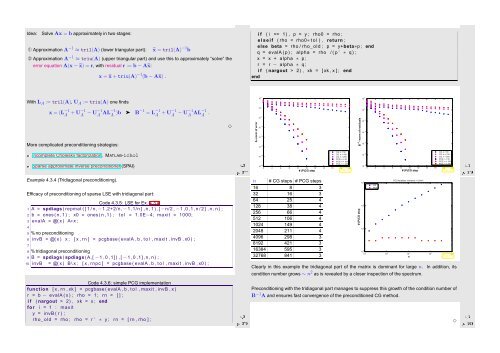
Example 4.3.4 (Tridiagonal preconditioning).
Efficacy of preconditioning of sparse LSE with tridiagonal part:
Code 4.3.5: LSE for Ex. 4.3.4
1 A = spdiags ( repmat ( [ 1 / n, −1 ,2+2/n, −1 ,1/n ] , n , 1 ) ,[−n/2 , −1 ,0 ,1 ,n / 2 ] , n , n ) ;
2 b = ones ( n , 1 ) ; x0 = ones ( n , 1 ) ; t o l = 1.0E−4; maxit = 1000;
3 evalA = @( x ) A∗x ;
4
5 % no preconditioning
6 invB = @( x ) x ; [ x , rn ] = pcgbase ( evalA , b , t o l , maxit , invB , x0 ) ;
7
8 % tridiagonal preconditioning
9 B = spdiags ( spdiags (A,[ − 1 ,0 ,1]) ,[ −1 ,0 ,1] ,n , n ) ;
10 invB = @( x ) B \ x ; [ x , rnpc ] = pcgbase ( evalA , b , t o l , maxit , invB , x0 ) ;
n # CG steps # PCG steps
16 8 3
32 16 3
64 25 4
128 38 4
256 66 4
512 106 4
1024 149 4
2048 211 4
4096 298 3
8192 421 3
16384 595 3
32768 841 3
# (P)CG step
PCG iterations: tolerance = 0.0001
CG
PCG
10 2
10 1
10 0
10 1 10 2 10 3 10 4 10 5
n
Fig. 54
10 3
Clearly in this example the tridiagonal part of the matrix is dominant for large n.
condition number grows ∼ n 2 as is revealed by a closer inspection of the spectrum.
In addition, its
Code 4.3.6: simple PCG implementation
1 function [ x , rn , xk ] = pcgbase ( evalA , b , t o l , maxit , invB , x )
2 r = b − evalA ( x ) ; rho = 1 ; rn = [ ] ;
3 i f ( nargout > 2) , xk = x ; end
4 for i = 1 : maxit
5 y = invB ( r ) ;
6 rho_old = rho ; rho = r ’ ∗ y ; rn = [ rn , rho ] ;
Ôº¿ º¿
Preconditioning with the tridiagonal part manages to suppress this growth of the condition number of
B −1 A and ensures fast convergence of the preconditioned CG method.
Ôº¿¼ º¿
✸