Numerical Methods Contents - SAM

y
y 1
y(t)
y 0
t
t 0 t 1 Fig. 133
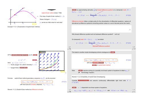
explicit Euler method (Euler 1768)
✁ First step of explicit Euler method (d = 1):
Slope of tangent = f(t 0 ,y 0 )
y 1 serves as initial value for next step!
(11.2.1) by approximating derivative
dt d by forward difference quotient on a (temporal) mesh M :=
{t 0 , t 1 ,...,t N }:
ẏ = f(t,y) ←→
y k+1 − y k
h k
= f(t k ,y h (t k )) , k = 0,...,N − 1 . (11.2.2)
Difference schemes follow a simple policy for the discretization of differential equations: replace all
derivatives by difference quotients connecting solution values on a set of discrete points (the mesh).
Example 11.2.1 (Visualization of explicit Euler method).
△
Why forward difference quotient and not backward difference quotient?
Let’s try!
Ôº½ ½½º¾
On (temporal) mesh M := {t 0 , t 1 ,...,t N } we obtain
ẏ = f(t,y) ←→
y k+1 − y k
h k
= f(t k+1 ,y h (t k+1 )) , k = 0,...,N − 1 . (11.2.3)
Backward difference quotient
Ôº¿ ½½º¾
2.4
2.2
exact solution
explicit Euler
This leads to another simple timestepping scheme analoguous to (11.2.1):
IVP for Riccati differential equation, see Ex. 11.1.4
2
1.8
ẏ = y 2 + t 2 . (11.1.6)
Here: y 0 = 1 2 , t 0 = 0, T = 1, ✄
— ˆ= “Euler polygon” for uniform timestep h = 0.2
↦→ ˆ= tangent field of Riccati ODE
y
1.6
1.4
1.2
1
0.8
0.6
0.4
0 0.2 0.4 0.6 0.8 1 1.2 1.4
t
Fig. 134
✸
y k+1 = y k + h k f(t k+1 ,y k+1 ) , k = 0,...,N − 1 , (11.2.4)
with local timestep (stepsize) h k := t k+1 − t k .
(11.2.4) = implicit Euler method
Note: (11.2.4) requires solving of a (possibly non-linear) system of equations to obtain y k+1 !
(➤ Terminology “implicit”)
Formula:
explicit Euler method generates a sequence (y k ) N k=0 by the recursion
y k+1 = y k + h k f(t k ,y k ) , k = 0,...,N − 1 , (11.2.1)
with local (size of) timestep (stepsize) h k := t k+1 − t k .
Remark 11.2.2 (Explicit Euler method as difference scheme).
Ôº¾ ½½º¾
Remark 11.2.3 (Feasibility of implicit Euler timestepping).
Consider autonomous ODE and assume continuously differentiable right hand side: f ∈
C 1 (D, R d ).
Ôº ½½º¾
y k+1 = y k + h k f(t k+1 ,y k+1 ) ⇔ G(h,y k+1 ) = 0 with G(h,z) := z − hf(z) − y k .
(11.2.4) ↔ h-dependent non-linear system of equations: