Numerical Methods Contents - SAM

Proof. Straightforward computation, see (7.2.4).
✷
Idea: (7.2.7) ➣ z = F −1 n diag(F n u)F n x
Conclusion
(from F n = nF −1 n ):
C = F−1 n diag(d 1 , . ..,d n )F n . (7.2.7)
Lemma 7.2.2, (7.2.7) ➣ multiplication with Fourier-matrix will be crucial operation in algorithms for
circulant matrices and discrete convolutions.
Therefore this operation has been given a special name:
Code 7.2.6: discrete periodic convolution:
straightforward implementation
1 function z=pconv ( u , x )
2 n = length ( x ) ; z = zeros ( n , 1 ) ;
3 for i =1:n , z ( i ) =dot ( conj ( u ) ,
x ( [ i : −1:1 ,n:−1: i + 1 ] ) ) ;
4 end
Code 7.2.8: discrete periodic convolution: DFT
implementation
1 function z= p c o n v f f t ( u , x )
2 z = i f f t ( f f t ( u ) .∗ f f t ( x ) ) ;
Definition 7.2.3 (Discrete Fourier transform (DFT)).
The linear map F n : C n ↦→ C n , F n (y) := F n y, y ∈ C n , is called discrete Fourier transform
(DFT), i.e. for c := F n (y)
n−1 ∑
c k =
j=0
y j
Ôº º¾
ωn kj , k = 0, ...,n − 1 . (7.2.8)
Rem. 7.1.6:
discrete convolution of n-vectors (→ Def. 7.1.1) by periodic discrete convolution of 2n−
1-vectors (obtained by zero padding):
Ôº º¾
Recall the convention also relevant for the discussion of the DFT: vector indexes range from 0 to
n − 1!
Terminology: c = F n y is also called the (discrete) Fourier transform of y
MATLAB-functions for discrete Fourier transform (and its inverse):
Implementation of
discrete convolution (→
Def. 7.1.1) based on
periodic discrete convolution ✄
Built-in MATLAB-function:
y = conv(h,x);
Code 7.2.9: discrete convolutiuon: DFT implementation
1 function y = myconv ( h , x )
2 n = length ( h ) ;
3 % Zero padding
4 h = [ h ; zeros ( n−1,1) ] ; x =
[ x ; zeros ( n−1,1) ] ;
5 % Periodic discrete convolution of length 2n − 1
6 y = p c o n v f f t ( h , x ) ;
DFT: c=fft(y) ↔ inverse DFT: y=ifft(c);
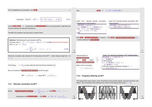
7.2.2 Frequency filtering via DFT
7.2.1 Discrete convolution via DFT
The trigonometric basis vectors, when interpreted as time-periodic signals, represent harmonic oscillations.
This is illustrated when plotting some vectors of the trigonometric basis (n = 16):
1
Fourier−basis vector, n=16, j=1
1
Fourier−basis vector, n=16, j=7
1
Fourier−basis vector, n=16, j=15
0.8
0.8
0.8
multiplication with circulant matrix (→ Def. 7.1.3) z = Cx, C := ( ) n
Ôº º¾
u i−j i,j=1 .
Recall discrete periodic convolution z k = n−1 ∑
u k−j x j (→ Def. 7.1.2), k = 0, ...,n − 1
j=0
↕
Value
0.6
0.4
0.2
0
−0.2
−0.4
−0.6
Value
0.6
0.4
0.2
0
−0.2
−0.4
−0.6
Value
0.6
0.4
0.2
0
−0.2
−0.4
−0.6
Ôº º¾
−0.8
Real part
Imaginary p.
−0.8
Real part
Imaginary p.
−0.8
Real part
Imaginary p.