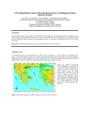
76 Fig. 15: Artistic view of the upcoming ESA-mission SWARM that will consist of a three-satellite constellation measuring the geomagnetic field. Die kommende ESA-Mission SWARM wird mit einer Konstellation aus drei Satelliten das Erdmagnetfeld vermessen – modellhafte Darstellung. Swarm mission (Fig. 15). Three satellites will be launched in 2009 and are intended to measure the magnetic field and its variations far more accurately than ever before (Friis-Christensen et al., <strong>2004</strong>). Based on the expertise gained from CHAMP, <strong>GFZ</strong> is well prepared to play a leading role in this ambitious mission. Acknowledgments Parts of the work described here have been funded by the „BMBF/DFG Sonderprogramm GEOTECHNOLOGIEN“, the DFG „Schwerpunktprogramm Erdmagnetische Variationen“, or have been carried out within the „INKABA YE AFRICA“ project. The results presented were possible only by the data acquisition and processing work of CHAMP data, Sungchang Choi and Wolfgang Mai, and German repeat station and observatory data, Martin Fredow, Anneleen Glodeck, Ingrid Goldschmidt, Jürgen Haseloff, Carsten Müller, Hannelore Podewski, Stefan Rettig, Jutta Schulz, Manfred Schüler, and Kathrin Tornow. All maps were plotted using the GMT software (Wessel and Smith, 1991). References Amm, O. and A. Viljanen, Ionospheric disturbance magnetic field continuation from the ground to the ionosphere using spherical elementary current systems, Earth Planets Space, 51, 431-440, 1999. Campbell, W.H., Introduction to geomagnetic fields, Cambridge University Press, 290 pp., 1997. Chambodut, A. and M. Mandea, Evidence for geomagnetic jerks in comprehensive models, Earth Planets Space, 57, 139-149, <strong>2005</strong>. Friis-Christensen, E., A. De Santis, A. Jackson, G. Hulot, A. Kuvshinov, H. Lühr, M. Mandea, S. Maus, N. Olsen, M. Purucker, M. Rother, T. Sabaka, A. Thomson, S. Vennerstrom, and P. Visser, Swarm. The Earth's Magnetic Field and Environment Explorers, ESA SP-1279, 6, <strong>2004</strong>. Hulot, G., C. Eymin, B. Langlais, M. Mandea, and N. Olsen, Small-scale structure dynamics of the geodynamo inferred from Ørsted and MAGSAT satellite data, Nature, 416, 620- 623, 2002. Jackson, A., A. R. T. Jonkers and M. R. Walker, Four centuries of geomagnetic secular variation from historical records, Phil. Trans. R. Soc. Lond., A, 358, 975-990. Langel, R. A., R. H. Estes, G. D. Mead, E. B. Fabiano, and E. R. Lancaster, Initial geomagnetic field model from Magsat vector data, Geophys. Res. Lett., 7(10), doi: 10.1029/0GPRLA000007000010000793000001, issn: 0094-8276, 1980. Langlais, B. and M. Mandea, An IGRF candidate main geomagnetic field model for epoch 2000 and a secular variation model for 2000-<strong>2005</strong>, Earth Planets Space, 52pp, 1137-1148, 2000. Mandea, M. and S. Macmillan, International Geomagnetic Reference Field – the eighth generation, Earth Planets Space, 52, 1119-1124, 2000. Mandea, M. and M. Purucker, Measurements of the Earth’s magnetic field from space, Surveys in Geophysiscs, 26, (No. 4), 415-459, DOI: 10.1007/s10712-005- 3857-x, <strong>2005</strong>. Maus, S., S. Maxmillan, T. Chernova, S. Choi, D. Dater, V. Golovkov, V. Lesur, F. Lowes, H. Lühr, W. Mai, S. McLean, N. Olsen, M. Rother, T. Sabaka, A. Thomson und T. Zvereva, The 10 th Generation International Geomagnetic Reference Field, Geophys. J. Int., 161, 561-656, <strong>2005</strong>. Maus, S., M. Rother, K. Hemant, C. Stolle, H. Lühr, A. Kuvshinov, and N. Olsen, Earth's lithospheric magnetic field determined to spherical harmonic degree 90 from CHAMP satellite measurements, Geophys. J. Int., doi: 10.1111/j.1365- 246X.<strong>2005</strong>.02833.x, 2006. Olsen, N., H. Lühr, T. Sabaka, M. Mandea, M. Rother, L. Toffner-Clausen, S. Choi, CHAOS - A Model of Earth’s Magnetic Field derived from CHAMP, Ørsted, and SAC-C magnetic satellite data, J. Geophys. Int., in review, 2006. Olsen, N., L. Toffner-Clausen, T. J. Sabaka, P. Brauer, J. G. Merayo, J. L. Jorgensen, J.-M. Leger, O. V. Nielsen, F. Primdahl, and T. Risbo, Calibration of the Ørsted vector magnetometer, Earth Planet Space, 55, 11-18, 2003. Ritter, P., H. Lühr, A. Viljanen, O. Amm, A. Pulkkinen, and I. Sillanpää, Ionospheric currents estimated simultaneously from CHAMP satellite and IMAGE ground-based magnetic field measurements: A statistical study at auroral latitudes, Ann. Geophys., 22, 417-430, <strong>2004</strong>. Sabaka, T., N. Olsen, and R. A. Langel, A comprehensive model of the quiet-time, near-Earth magnetic field: phase 3, Geophys. J. Int, 151, 32-68, 2002. Sabaka, T., N. Olsen, and M.E. Purucker, Extending comprehensive models of the Earth’s magnetic field with Ørsted and CHAMP data, Geophys. J. Int., 159, 521- 547, <strong>2004</strong>. Thébault, E., J. J. Schott, M. Mandea, and J. P. Hoffbeck, A new proposal for Spherical Cap Harmonic modelling, Geophys. J. Int., 159, 83-103, <strong>2004</strong>. Wardinski, I., Core Surface Flow Models from Decadal and Subdecadal Secular Variation of the Main Geomagnetic Field, Ph.D., FU Berlin, 132 pp, <strong>2005</strong>. Wessel, P. and W. H. F. Smith, New, improved version of the Generic Mapping Tools released, EOS Trans. AGU, 79 579, 1998. <strong>Zweijahresbericht</strong> <strong>2004</strong>/<strong>2005</strong> GeoForschungsZentrum Potsdam
CONTINENT – Der Baikalsee: ein außergewöhnliches kontinentales Klimaarchiv Hedi Oberhänsli, Birgit Heim, François Demory, Jens Klump, Hermann Kaufmann, Norbert Nowaczyk, Ronald Conze und CONTINENT-Partner Lake Baikal represents one of the few Eurasian, continental, lacustrine sites with an extremely long, uninterrupted sedimentary record (spanning potentially 25 million years) that can be exploited for high-resolution palaeoclimate studies. Baikal is also close to the boundaries of two important weather systems - the Siberian high-pressure zone and the Asian monsoon zone. Over recent decades, scientists have become increasingly aware that weather systems in one region of the world can have significant effects on climate elsewhere, many thousands of miles away. By definition, remote influences such as these are termed teleconnections. Moreover, it is also increasingly apparent that the earth's climate can change very abruptly in contrast to current predictions that, for example, global warming will occur gradually over the next 50 to 100 years. It is therefore important that we are fully able to understand the extent and rate of change of past climate variability. Lake Baikal represents a site remote from oceanic influences, for long time ignored in highresolution climate studies. By reconstructing climate variability in continental Eurasia, we can contribute to the knowledge base of, for example, the importance of changes in oceanic circulation to climate in regions remote from oceans during known periods of instability. In CONTINENT (High Resolution CONTINENTal Paleoclimate Record in Lake Baikal) we used both biological and non-biological proxies to reconstruct climate variability in Eurasia during the interglacials known as the Holocene (10 kiloannum (ka = 1000 years) before present BP) and the Eemian (c. 110 to130 ka BP), and the preceding Terminations I and II phases. Of interest were also abrupt climatic changes, in particular their timing and extent. However, in order to do this with confidence we also investigated contemporary processes in the lake that are likely to affect each of the different climate proxies. Challenges identified include understanding: (i) biological processes in the photic zones, e.g. life cycle strategies of organisms dependent on ice-cover in the lake; (ii) processes influencing windblown and riverine input to the lake; (iii) transport of biological and non-biological particles through the water column, e.g. rates of transport, seasonality; and (iv) processes that affect final incorporation of sediment particles into the sedimentary record, e.g. grazing, dissolution of diatom tests, bacterial consumption of organic material, typical processes occurring at the water/sediment interface. In order to address these challenges, climate has been reconstructed at high resolution: on decadal to centennial scales. Using these results we have learned more about the influence of climate forcing factors and their feedbacks. CONTINENT provided an improved knowledge on the central Asian climate history, which helps toward a better understanding of European and Northern Hemisphere climate systems. Meteorologische Messreihen belegen, dass auch Zentraleurasien in den letzten 100 Jahren eine deutliche Erwärmung erfahren hat, die sich wahrscheinlich in die Zukunft fortsetzen wird (Todd und Mackay, <strong>2004</strong>). Diese Aussagen beruhen auf Eisdickenentwicklung am Baikalsee und dem Beginn des Eisaufbaus und Abschmelzens. Temperaturmessungen zeigen weiter, dass seit den 1980er Jahren ansteigende kontinentale Wintertemperaturen über Eurasien und Nordamerika zu einem großen Teil für die beobachtete generelle Erwärmung über der Nordhemisphäre verantwortlich sind, während der Nordatlantik leicht kühlere Werte zeigt. In Sibirien hat das zu extremen räumlich und zeitlich gestreuten Temperatur- und Feuchtigkeitsanomalien geführt. Weite Permafrostbereiche finden sich bereits klimatisch im Ungleichgewicht. Bleibt es bei diesem Klimatrend, würde das bedeuten, dass sich die Grenze des permanenten Dauerfrostes, die sich derzeit noch am Nordende des Baikalsees befindet, langsam aber stetig weiter nach Norden zurückzieht. Dies wird eine Vielzahl von ökologischen Veränderungen nach sich ziehen. Noch ungeklärt ist, inwieweit die Auftauprozesse in Permafrostböden, unter anderem durch einsetzende Kompostierung der organischen Substanzen, Treibhausgase in noch nicht einschätzbarem Ausmaß zur Klimaveränderung freisetzen werden. Dass sie ihre Bedeutung haben, deckt sich mit Modellen, denn deren Ergebnisse gehen von starken Zunahmen von Treibhausgas und partikulären Aerosolen aus. Aus klimatischen Modellierungen wird prognostiziert, dass in den nächsten Dekaden in Zentralasien die Wintertemperaturen um 2 bis 8 °C (globale Durchschnittstemperaturen 1,5 bis 4,5 °C) ansteigen und die Niederschläge um 300 bis 600 mm/Jahr zunehmen könnten (IPCC, 2001; z. B. Abb. 1). Die für die nächsten 50 bis 150 Jahre vorliegenden Prognosen sind allerdings mit großer Unsicherheit behaftet, weil Rückkopplungsprozesse nicht ausreichend bekannt sind. Ebenfalls sind in Zukunft mehr Extremereignisse zu erwarten. In Zentralsibirien würde das bedeuten, dass mehr Frühjahrs- und Sommerstürme auftreten, die zu extremen Sommergewittern führen und verstärkt massive Staubmassen aus den zentralasiatischen Wüsten nach Osten bis nach Nordamerika transportieren. <strong>Zweijahresbericht</strong> <strong>2004</strong>/<strong>2005</strong> GeoForschungsZentrum Potsdam 77
- Seite 1 und 2:
Zweijahresbericht GeoForschungsZent
- Seite 3 und 4:
Inhaltsverzeichnis Vorwort III Einl
- Seite 5 und 6:
Vorwort Der vorliegende Zweijahresb
- Seite 7 und 8:
Das System Erde - Forschungsgegenst
- Seite 9 und 10:
Geodynamische Prozesse sind als rä
- Seite 11 und 12:
Abb. 4: Geophysikalisches Observato
- Seite 13 und 14:
GFZ beteiligt sich maßgeblich im F
- Seite 15 und 16:
GITEWS - German-Indonesian Tsunami
- Seite 17 und 18:
die Simulationen auf eine gesichert
- Seite 19 und 20:
Abb. 8: Verteilung der Tsunami Boje
- Seite 21 und 22:
Abb. 10: Schematischer Aufbau des G
- Seite 23 und 24:
ten sind in thematischen Gruppen or
- Seite 25 und 26:
Das Bam-Erdbeben 2003: Präzise Her
- Seite 27 und 28:
so dass man hier ein komplexeres St
- Seite 29 und 30:
Abb. 4: Berechnete Bodenverformunge
- Seite 31 und 32:
Diskussion und Schlußfolgerungen D
- Seite 33 und 34:
Wang, R., Xia, Y., Grosser, H., Wet
- Seite 35 und 36:
D-INSAR-Forschung in China: Monitor
- Seite 37 und 38:
Abb. 3: Auswirkung von Absenkungen:
- Seite 39 und 40: Abb. 6: Mit Nivellement gemessene A
- Seite 41 und 42: Abb. 10a bis c: Durchschnittliche B
- Seite 43 und 44: Prozesse, die die Anden formten - 1
- Seite 45 und 46: 80 Dissertationsprojekten über 15
- Seite 47 und 48: wurde mit den gleichen Apparaturen,
- Seite 49 und 50: dung, die sich von der seismisch be
- Seite 51 und 52: Abb. 9: Die linke Abbildung zeigt d
- Seite 53 und 54: Abb. 11: Korrelation verschiedener
- Seite 55 und 56: (vgl. Abb. 13). Die Zentralen Anden
- Seite 57 und 58: 6 Mill. Jahren gesteuert worden. Zu
- Seite 59 und 60: Schurr, B., A. Rietbrock, G. Asch,
- Seite 61 und 62: „Inkaba ye Africa“ - dem dynami
- Seite 63 und 64: von Meeresströmungen, die klimatis
- Seite 65 und 66: Entwicklung der Kontinentalränder
- Seite 67 und 68: CHAMP und GRACE - erfolgreiche Schw
- Seite 69 und 70: sie bereits mehr als 21000-mal die
- Seite 71 und 72: Abb. 6: C 20-Variation abgeleitet a
- Seite 73 und 74: Abb. 10a, b: Zeitserie der Beckenmi
- Seite 75 und 76: Abb. 14: Zwei Ausschnitte aus der K
- Seite 77 und 78: A comprehensive view of the Earth
- Seite 79 und 80: Fig. 2: Participants of the interna
- Seite 81 und 82: Fig. 4: Orienting a first prototype
- Seite 83 und 84: Fig. 6: Coverage of the Earth with
- Seite 85 und 86: Fig. 7: Percentage change of the ge
- Seite 87 und 88: Fig. 10: Two teams from GFZ Potsdam
- Seite 89: observatories Fürstenfeldbruck, Ni
- Seite 93 und 94: wird das südliche Einzugsgebiet de
- Seite 95 und 96: masignale im Sediment ab. Der Baika
- Seite 97 und 98: Abb. 6: Ausstattung der Sedimentfal
- Seite 99 und 100: Abb. 8: Chlorophyll-a-Konzentration
- Seite 101 und 102: optischen Rahmenbedingungen, die du
- Seite 103 und 104: Abb. 13: Häufigkeit des Chl-a, sow
- Seite 105 und 106: Am GFZ Potsdam wurden die Kerne gem
- Seite 107 und 108: (Biome) evaluiert (Prentice et al.,
- Seite 109 und 110: Maerki, M., Müller, B., Wehrli, B.
- Seite 111 und 112: Seismische Vorauserkundung im Tunne
- Seite 113 und 114: Abb. 2: Seismogramme der numerische
- Seite 115 und 116: Abb. 5: Daten nach Bearbeitung (Emp
- Seite 117 und 118: Technologieentwicklung im In-Situ-
- Seite 119 und 120: Abb. 2: Geologisches Blockbild der
- Seite 121 und 122: Abb. 4: Das Abbild der elektrischen
- Seite 123 und 124: Rissleitfähigkeit von 1 Dm hin. Di
- Seite 125 und 126: ge Nutzung eines Heißwasserreservo
- Seite 127 und 128: Hochdruck-Mineralphysik mit Synchro
- Seite 129 und 130: innerhalb von Druckkammern mit hohe
- Seite 131 und 132: zur Probe durch intransparente Stem
- Seite 133 und 134: Druckmessung Mineralphysikalische H
- Seite 135 und 136: am Probenende sollte die Energie m
- Seite 137 und 138: Abb. 14: Ultraschall-Daten-Transfer
- Seite 139 und 140: Abb. 18: Elastische Wellengeschwind
- Seite 141 und 142:
Abb. 22: Transiente Messungen am Qu
- Seite 143 und 144:
gramm MgSiO 3 (Angel & Hugh-Jones,
- Seite 145 und 146:
Abb. 30: Weltweite Entwicklung der
- Seite 147 und 148:
Woodland, A.B., Angel, R.J. (1997).
- Seite 149 und 150:
Neue experimentelle Entwicklungen a
- Seite 151 und 152:
Abb. 3: Tiefenprofil einer Referenz
- Seite 153 und 154:
A B Abb.5:SIMS-Kalibrierungskurven
- Seite 155 und 156:
Risikokarten für Deutschland: erst
- Seite 157 und 158:
Da die Auswirkungen der meisten Nat
- Seite 159 und 160:
Abb. 4:A: Choroplethenkarte des auf
- Seite 161 und 162:
ERA-40 Daten des ECMWF gewonnen. Mi
- Seite 163 und 164:
Abb. 9: Mittlere Wohngebäudezusamm
- Seite 165 und 166:
Kaplan, S., Garrick, B. J.: On the
- Seite 167 und 168:
Das Industrie-Partnerschaftprogramm
- Seite 169 und 170:
Abb. 2: Vier grundlegende Elemente
- Seite 171 und 172:
Abb. 5: Die Analyse von Muttergeste
- Seite 173 und 174:
den als Untersuchungsgebiet ausgew
- Seite 175 und 176:
tionskinetischen Modellen, welche e
- Seite 177 und 178:
Zweijahresbericht 2004/2005 GeoFors
- Seite 179 und 180:
Department 1 Geodäsie und Fernerku
- Seite 181 und 182:
Die am GFZ-Analysezentrum erzeugten
- Seite 183 und 184:
Abb. 1.6: Mittelwerte der von GFZ u
- Seite 185 und 186:
Tabelle 1.1:Residuen zur kombiniert
- Seite 187 und 188:
gression der Vergletscherung in die
- Seite 189 und 190:
Abb 1.17: Aus den am 30.07. (oben)
- Seite 191 und 192:
Validierung der mittels GPS vermess
- Seite 193 und 194:
Abb. 1.24: Die geografische Verteil
- Seite 195 und 196:
Vergleich der zeitlichen Variatione
- Seite 197 und 198:
Abb. 1.33: Globale und regional ver
- Seite 199 und 200:
Abb. 1.35: Vergleich von GPS-Okkult
- Seite 201 und 202:
weltweit verteilten Stationen werde
- Seite 203 und 204:
wicklung divergieren die Abschätzu
- Seite 205 und 206:
im Wärmehaushalt zurückgeführt w
- Seite 207 und 208:
zungsmethode und dem Grad der Kugel
- Seite 209 und 210:
a) b) Die Zone der niedrigen Dichte
- Seite 211 und 212:
a) b) Abb. 1.54: (A) Ein erstes Dic
- Seite 213 und 214:
Abb. 1.58: Alternative geodynamisch
- Seite 215 und 216:
kungen und hydrologischen Effekten
- Seite 217 und 218:
strömen mit dem Abfluss in die Amu
- Seite 219 und 220:
Fernerkundung Die Fernerkundung ste
- Seite 221 und 222:
schen Arten deutlich im Sichtbaren
- Seite 223 und 224:
Abb. 1.75: Skalierungsexperiment: a
- Seite 225 und 226:
Abb. 1.78: Spektrale Varianten von
- Seite 227 und 228:
endgültigen Simulationsspektren er
- Seite 229 und 230:
Department 2 Physik der Erde Die Br
- Seite 231 und 232:
Abb. 2.2: Temporäre Station Dissel
- Seite 233 und 234:
strukturen im direkten Umfeld des G
- Seite 235 und 236:
Abb. 2.8: Microarray-Messungen in I
- Seite 237 und 238:
Vulkanismus und Erdbeben Einer mitt
- Seite 239 und 240:
und Gefährdungspotenzial der Erde
- Seite 241 und 242:
Abb. 2.19: Modell des Aufstiegs von
- Seite 243 und 244:
Abb. 2.22: Das Seismometer der Stat
- Seite 245 und 246:
Abb. 2.26: Im Berichtszeitraum fand
- Seite 247 und 248:
Abb. 2.29: Verteilung des elektrisc
- Seite 249 und 250:
Abb. 2.31: Beispiel eines tomograph
- Seite 251 und 252:
Abb. 2.33: (a) bis (c) Wachsendes P
- Seite 253 und 254:
Abb. 2.35: Illustration des neuen M
- Seite 255 und 256:
Methode der Receiver Funktionen ist
- Seite 257 und 258:
Abb. 2.42: Untergrenze der afrikani
- Seite 259 und 260:
überwiegend in Europa und dem Mitt
- Seite 261 und 262:
für alle geologischen Erscheinungs
- Seite 263 und 264:
Abb. 2.51b: Sicher ist sicher! Vors
- Seite 265 und 266:
Vor der wissenschaftlichen Modellie
- Seite 267 und 268:
Abb. 2.57: Teilnehmer des Festkollo
- Seite 269 und 270:
y eine Messkampagne an 40 Säkularp
- Seite 271 und 272:
nen aus Modellrechnungen, mit welch
- Seite 273 und 274:
kurz bevor geomagnetische Jerks beo
- Seite 275 und 276:
Anhand von Archiven kosmogener Nukl
- Seite 277 und 278:
Abb. 2.68: Globale Verteilung der i
- Seite 279 und 280:
der linken Seite der Abb. 2.70 entn
- Seite 281 und 282:
Kind, R., X. Yuan, J. Saul, D. Nels
- Seite 283 und 284:
Zweijahresbericht 2004/2005 GeoFors
- Seite 285 und 286:
Department 3 Geodynamik Tektonische
- Seite 287 und 288:
Abb. 3.3: Datierung der Spät-Pleis
- Seite 289 und 290:
geführt. Ausgehend von ‚state of
- Seite 291 und 292:
zu setzen und Vorhersagestrategien
- Seite 293 und 294:
Bruchentstehung und Bruchausbreitun
- Seite 295 und 296:
Abb. 3.10: Oben Mitte: Ummantelte G
- Seite 297 und 298:
Abb. 3.15: Oben: Topographische Kar
- Seite 299 und 300:
Abb. 3.17: (a) Modellaufbau des num
- Seite 301 und 302:
Abb. 3.20 zeigt die Permeabilität
- Seite 303 und 304:
auch in allen diesen Fällen noch a
- Seite 305 und 306:
Abb. 3.26: Dokumentation eines Dür
- Seite 307 und 308:
Abb. 3.29: Lage des El’gygytgyn I
- Seite 309 und 310:
weniger (Kaltzeiten) verdünnt. Da
- Seite 311 und 312:
Zweijahresbericht 2004/2005 GeoFors
- Seite 313 und 314:
Department 4 Chemie der Erde Geodyn
- Seite 315 und 316:
Abb.4.3:Experimentell bestimmte B-I
- Seite 317 und 318:
System H2O-NaCl-B 2O 3 bei 400 °C/
- Seite 319 und 320:
Abb. 4.9: (a) Brom-Konzentrationen
- Seite 321 und 322:
Abb. 4.13: Zr-, U- und Pb-Molalitä
- Seite 323 und 324:
Abb. 4.16: Spurenelementverteilungs
- Seite 325 und 326:
durch Fluide produzierten Mikrophas
- Seite 327 und 328:
Abb. 4.21: (a) HRTEM-Aufnahme einer
- Seite 329 und 330:
stark richtungsabhängig ist. Unser
- Seite 331 und 332:
Abb. 4.28: KTB-Lokation von einem L
- Seite 333 und 334:
Abb. 4.30: Horizontaler Schnitt ein
- Seite 335 und 336:
analysiert. Um das Verhalten der Sp
- Seite 337 und 338:
sehr weiten Bereich des Erdmantels
- Seite 339 und 340:
Abb. 4.37: Das lichtoptische Bild z
- Seite 341 und 342:
Abb. 4.40: (a) Zylindrische Probe e
- Seite 343 und 344:
Abb. 4.43: Rückgestreute Elektrone
- Seite 345 und 346:
Abb.4.46:Mit zunehmender Probenlän
- Seite 347 und 348:
nen Richtungen bestimmt. In Abb. 4.
- Seite 349 und 350:
Abb.4.53:Scher- und adiabatisches K
- Seite 351 und 352:
Abb. 4.56: Aufbau des Experiments z
- Seite 353 und 354:
Signaturen radiogener Isotope, v. a
- Seite 355 und 356:
Abb. 4.60: Nd (epsilon Nd)- und Sr-
- Seite 357 und 358:
Das Zentraleuropäische Beckensyste
- Seite 359 und 360:
chergesteine der Skagerrak-Formatio
- Seite 361 und 362:
Abb. 4.71: Verteilung des Salzgehal
- Seite 363 und 364:
Abb. 4.74: Teufenplots ausgewählte
- Seite 365 und 366:
neuester Beckenmodellierungssoftwar
- Seite 367 und 368:
sowie die Modellierung des davon ab
- Seite 369 und 370:
ses Modell hat jahrzehntelang Anwen
- Seite 371 und 372:
Abb. 4.81: Lage des Untersuchungsge
- Seite 373 und 374:
Abb. 4.84: a) 3D Modell des Norwegi
- Seite 375 und 376:
Abb.4.86:Modellierte Druck- und Tem
- Seite 377 und 378:
Abb. 4.88: Foto der DEBITS Bohrloka
- Seite 379 und 380:
Abb. 4.90: Abhängigkeit der relati
- Seite 381 und 382:
Abb. 4.94: Lage der Bohrungen im Gu
- Seite 383 und 384:
führt. Neben dem GFZ Potsdam, Sekt
- Seite 385 und 386:
of highly evolved tin-granite magma
- Seite 387 und 388:
Department 5 Geoengineering Die Arb
- Seite 389 und 390:
Abb. 5.4: Anregung seismischer Impu
- Seite 391 und 392:
davor liegt die sog. Piora-Mulde, d
- Seite 393 und 394:
Abb. 5.12: Versuchsdeich mit seismi
- Seite 395 und 396:
Abb. 5.17: Verteilung von Salzstruk
- Seite 397 und 398:
Abb. 5.20: Geologischer Schnitt dur
- Seite 399 und 400:
Abb. 5.23: Bohrkerne aus der Weser-
- Seite 401 und 402:
Abb. 5.27: Schema einer „Fracture
- Seite 403 und 404:
Abb. 5.32: Epizentren katalogisiert
- Seite 405 und 406:
Abb. 5.35: Vulnerabilitäts-(Schade
- Seite 407 und 408:
isiko und wesentliche Teile zum Wer
- Seite 409 und 410:
ares Verhalten in Übereinstimmung
- Seite 411 und 412:
kreisregelung um Kegelachsen im Win
- Seite 413 und 414:
Abb. 5.45: Beispiele für die zeitl
- Seite 415 und 416:
Abb.5.50:Hochwasserwahrscheinlichke
- Seite 417 und 418:
Abb. 5.53: Jährlichkeiten der Rhei
- Seite 419 und 420:
schungsnetz Naturkatastrophen (DFNK
- Seite 421 und 422:
Das GFZ Potsdam auf einen Blick Nam
- Seite 423 und 424:
Gremien des GeoForschungsZentrums P
- Seite 425 und 426:
Abb. 3: Entwicklung der Ausbildungs
- Seite 427 und 428:
oberfläche, in den Meeren und in d
- Seite 429 und 430:
6. Modellierung: Die Modellierung k
- Seite 431 und 432:
• Einrichtung eines ICSU-Weltdate
- Seite 433 und 434:
Abb. 12: Entwicklung des Massendate
- Seite 435 und 436:
zone untersucht werden. Im Jahr 200
- Seite 437 und 438:
zu Impaktgläsern im Bohrlochtiefst
- Seite 439 und 440:
gen. Die OSG verwendete hierzu sowo
- Seite 441 und 442:
sich dabei in sehr ähnlichem Umfel
- Seite 443 und 444:
Abb. 30: Schematische Ansicht des I
- Seite 445 und 446:
jekten und tiefen Erdbebenbeobachtu
- Seite 447 und 448:
Prof. Dr. Günter Borm, Direktor de
- Seite 449 und 450:
Dipl.-Min. Marcus Wigand, „Geoche
- Seite 451 und 452:
Rayleigh wave tomography. Geophys.
- Seite 453 und 454:
zie Delta, Northwest Territories, C
- Seite 455 und 456:
Larter, S.R., di Primio, R. (2005):
- Seite 457 und 458:
Müller, H.-J., Schilling, F.R., La
- Seite 459 und 460:
Rybacki, E.; Dresen, G. (2004): Def
- Seite 461 und 462:
Bouguer gravity anomaly. Geophys. J
- Seite 463 und 464:
Glossar AAM Atmospheric Angular Mom