Skriptum zur Wahrscheinlichkeitstheorie

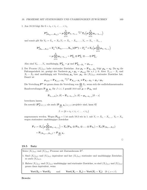
19. PROZESSE MIT STATIONÄREN UND UNABHÄNGIGEN ZUWÄCHSEN 169
1. Aus 18.10 folgt für 0 = t 0 < t 1 < . . . < t n
P µ (X t0 ,...,X tn ) = µ n ⊗
i=1
P ti−t i−1
19.3
= T n
(µ
n⊗ )
µ ti−t i−1
und somit gilt für Y 0 := Y t0 = X 0 , Y 1 := X t1 − X t0 , . . . , Y n := X tn − X tn−1
i=1
(
P µ (Y = T −1
0,...,Y n) n
(X t 0
, . . . , X tn )(P µ ) = T −1
n
◦ T n µ
= µ
n⊗
µ ti−t i−1
= P µ Y 0
⊗ P µ Y 1
⊗ . . . ⊗ P µ Y n
.
i=1
Also sind Y 0 , . . . , Y n unabhängig, P µ X 0
= µ und P µ X t−X s
= µ t−s .
n⊗ )
µ ti−t i−1
2. Der Prozess (X t ) t∈I habe stationäre Zuwächse. Aus µ t = P Xt−X 0
folgt µ 0 = ɛ 0 . Da ɛ 0 die
Faltungseinheit ist, genügt der Nachweis µ s ∗ µ t = µ s+t für s, t ≥ 0. Aber X s+t − X t und
X t − X 0 sind unabhängig mit Verteilung µ s bzw. µ t , da (X t ) t∈I stationäre Zuwächse hat.
Damit ist
10.18
µ s+t = P Xs+t −X 0
= P Xs,t−X t
∗ P Xt−X 0
= µ s ∗ µ t .
Die Verteilung P µ ist genau dann die Verteilung von ⊗ t∈I
X t , wenn sich die endlichdimensionalen
Randverteilungen P N X t
für J ⊂⊂ I gemäß 18.8 mit µ := P X0 und
berechnen lassen.
t∈J
i=1
P ti−1 ,t i
[x, B] = P ti−t i−1
[x, B] = µ ti−t i−1
[B − x]
Da sowohl (P µ J ) J⊂⊂I als auch (P N X t
) J⊂⊂I projektiv sind, kann Œ
t∈J
I := {0 = t 0 < t 1 < . . . < t n }
angenommen werden. Wegen P 0,0 = 1 ist nach 19.3 wie in 1. mit Y i := X ti − X ti−1 , Y 0 = X t0
wegen stationärer unabhängiger Zuwächse
19.5 Satz
P J := T n
(µ
n⊗
i=1
= P (Xt0 ,...,X tn ) = P N
) ( ) ( )
µ ti−t i−1
= T n PY0 ⊗ P Y1 ⊗ . . . ⊗ P Yn = Tn P(Y0,...,Y n)
X t
.
t∈J
Seien (X t ) t∈I und (Y t ) t∈I Prozesse mit Zustandsraum R d .
1. Sind (X t ) t∈I und (Y t ) t∈I äquivalent und hat (X t ) t∈I stationäre und unabhängige Zuwächse,
so auch (Y t ) t∈I .
2. Haben (X t ) t∈I und (Y t ) t∈I unabhängige und stationäre Zuwächse, so sind (X t ) t∈I und (Y t ) t∈I
genau dann äquivalent, wenn
VertX 0 = VertY 0 und Vert(X t − X s ) = Vert(Y t − Y s ) (0 ≤ s < t).
✷
Beweis: