Méthodes numériques en finance

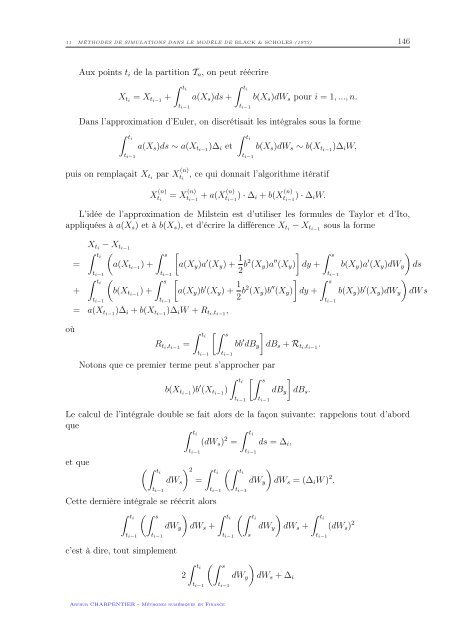
11 MÉTHODES DE SIMULATIONS DANS LE MODÈLE DE BLACK & SCHOLES (1973) 146
Aux points t i de la partition T n , on peut réécrire
X ti = X ti−1 +
∫ ti
∫ ti
a(X s )ds + b(X s )dW s pour i = 1, ..., n.
t i−1 t i−1
Dans l’approximation d’Euler, on discrétisait les intégrales sous la forme
∫ ti
t i−1
a(X s )ds ∼ a(X ti−1 )∆ i et
∫ ti
t i−1
b(X s )dW s ∼ b(X ti−1 )∆ i W,
puis on remplaçait X ti
par X (n)
t i
, ce qui donnait l’algorithme itératif
X (n)
t i
= X (n)
t i−1
+ a(X (n)
t i−1
) · ∆ i + b(X (n)
t i−1
) · ∆ i W.
L’idée de l’approximation de Milstein est d’utiliser les formules de Taylor et d’Ito,
appliquées à a(X s ) et à b(X s ), et d’écrire la différence X ti − X ti−1 sous la forme
=
+
X ti − X ti−1
∫ ti
(
t i−1
∫ ti
(
t i−1
a(X ti−1 ) +
b(X ti−1 ) +
∫ s
[
t i−1
∫ s
t i−1
[
= a(X ti−1 )∆ i + b(X ti−1 )∆ i W + R ti ,t i−1
,
a(X y )a ′ (X y ) + 1 ]
2 b2 (X y )a ′′ (X y )
a(X y )b ′ (X y ) + 1 ]
2 b2 (X y )b ′′ (X y )
dy +
dy +
∫ s
)
b(X y )a ′ (X y )dW y ds
t i−1
)
b(X y )b ′ (X y )dW y dW s
t i−1
∫ s
où
R ti ,t i−1
=
∫ ti
[∫ s
]
bb ′ dB y dB s + R ti ,t i−1
.
t i−1 t i−1
Notons que ce premier terme peut s’approcher par
b(X ti−1 )b ′ (X ti−1 )
∫ ti
[∫ s
]
dB y dB s .
t i−1 t i−1
Le calcul de l’intégrale double se fait alors de la façon suivante: rappelons tout d’abord
que
et que
(∫ ti
∫ ti
t i−1
dW s
) 2
=
∫ ti
(dW s ) 2 = ds = ∆ i ,
t i−1 t i−1
∫ ti
Cette dernière intégrale se réécrit alors
∫ ti
(∫ s
)
dW y dW s +
t i−1 t i−1
(∫ ti
)
dW y dW s = (∆ i W ) 2 .
t i−1 t i−1
∫ ti
(∫ ti
)
dW y dW s +
t i−1
s
∫ ti
t i−1
(dW s ) 2
c’est à dire, tout simplement
∫ ti
(∫ s
)
2
dW y dW s + ∆ i
t i−1 t i−1
Arthur CHARPENTIER - Méthodes numériques en Finance