Méthodes numériques en finance

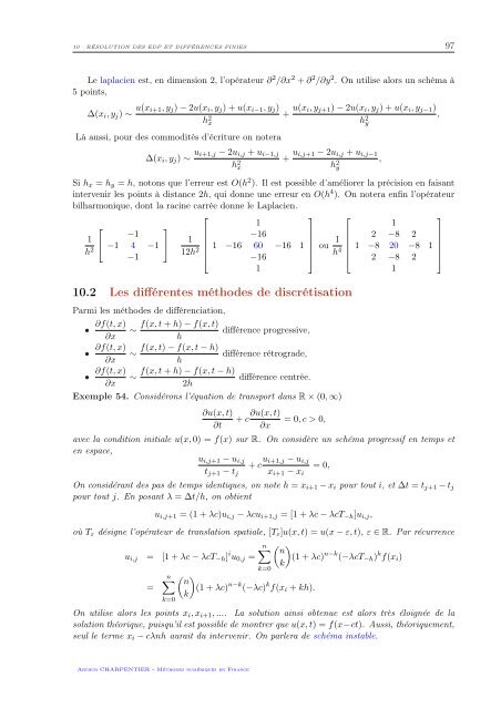
10 RÉSOLUTION DES EDP ET DIFFÉRENCES FINIES 97
Le laplacien est, en dimension 2, l’opérateur ∂ 2 /∂x 2 + ∂ 2 /∂y 2 . On utilise alors un schéma à
5 points,
∆(x i , y j ) ∼ u(x i+1, y j ) − 2u(x i , y j ) + u(x i−1 , y j )
h 2 x
Là aussi, pour des commodités d’écriture on notera
+ u(x i, y j+1 ) − 2u(x i , y j ) + u(x i , y j−1 )
h 2 ,
y
∆(x i , y j ) ∼ u i+1,j − 2u i,j + u i−1,j
h 2 x
+ u i,j+1 − 2u i,j + u i,j−1
h 2 ,
y
Si h x = h y = h, notons que l’erreur est O(h 2 ). Il est possible d’améliorer la précision en faisant
intervenir les points à distance 2h, qui donne une erreur en O(h 4 ). On notera enfin l’opérateur
bilharmonique, dont la racine carrée donne le Laplacien.
⎡
⎤ ⎡
⎤
⎡
⎤
1
1
−1
1
⎣
h 2 −1 4 −1 ⎦
1
−16
12h
−1
2 ⎢ 1 −16 60 −16 1
⎥
⎣ −16 ⎦ ou 1 2 −8 2
h 4 ⎢ 1 −8 20 −8 1
⎥
⎣ 2 −8 2 ⎦
1
1
10.2 Les différentes méthodes de discrétisation
Parmi les méthodes de différenciation,
∂f(t, x) f(x, t + h) − f(x, t)
• ∼ différence progressive,
∂x
h
∂f(t, x) f(x, t) − f(x, t − h)
• ∼ différence rétrograde,
∂x
h
∂f(t, x) f(x, t + h) − f(x, t − h)
• ∼ différence centrée.
∂x
2h
Exemple 54. Considérons l’équation de transport dans R × (0, ∞)
∂u(x, t)
∂t
∂u(x, t)
+ c = 0, c > 0,
∂x
avec la condition initiale u(x, 0) = f(x) sur R. On considère un schéma progressif en temps et
en espace,
u i,j+1 − u i,j
t j+1 − t j
+ c u i+1,j − u i,j
x i+1 − x i
= 0,
On considérant des pas de temps identiques, on note h = x i+1 − x i pour tout i, et ∆t = t j+1 − t j
pour tout j. En posant λ = ∆t/h, on obtient
u i,j+1 = (1 + λc)u i,j − λcu i+1,j = [1 + λc − λcT −h ]u i,j ,
où T ε désigne l’opérateur de translation spatiale, [T ε ]u(x, t) = u(x − ε, t), ε ∈ R. Par récurrence
n∑
( n
u i,j = [1 + λc − λcT −h ] i u 0,j = (1 + λc)
k)
n−k (−λcT −h ) k f(x i )
=
n∑
k=0
k=0
( n
k)
(1 + λc) n−k (−λc) k f(x i + kh).
On utilise alors les points x i , x i+1 , .... La solution ainsi obtenue est alors très éloignée de la
solution théorique, puisqu’il est possible de montrer que u(x, t) = f(x−ct). Aussi, théoriquement,
seul le terme x i − cλnh aurait du intervenir. On parlera de schéma instable.
Arthur CHARPENTIER - Méthodes numériques en Finance