Emissions Scenarios - IPCC

An Overview of Scenarios 201
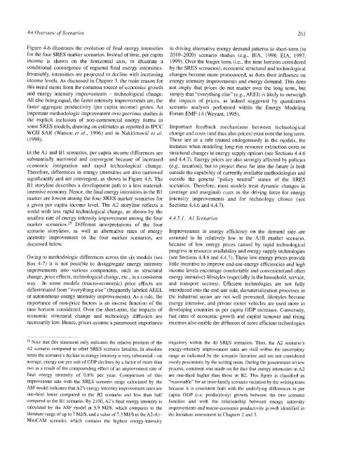
Figure 4-6 illustrates the evolution of final energy intensities
for the four SRES marker scenarios. Instead of time, per capita
income is shown on the horizontal axis, to illustrate a
conditional convergence of regional final energy intensities.
Invariably, intensities are projected to decline with increasing
income levels. As discussed in Chapter 3, the main reason for
this trettd stems from the common source of economic growth
and energy intensity improvements - technological change.
All else being equal, the faster intensity improvements are, the
faster aggregate productivity (per capita income) grows. An
important méthodologie improvement over previous studies is
the explicit inclusion of non-commercial energy forms in
some SRES models, drawing on estimates as reported in IPCC
WGII SAR (Watson et al., 1996) and in Nakicenovic et al.
(1998).
In the Al and ВI scenarios, per capita income differences are
substantially narrowed and convergent because of increased
economic integration and rapid technological change.
Therefore, differences in energy intensities are also narrowed
significantly and are convergent, as shown in Figure 4.6. The
Bl storyline describes a development path to a less materialintensive
economy. Hence, the final energy intensities in the В1
marker are lowest among the four SRES marker scenarios for
a given per capita income level. The A2 storyline reflects a
world with less rapid technological change, as shown by the
smallest rate of energy intensity improvement among the four
marker scenarios.Different interpretations of the four
scenario storylines, as well as alternative rates of energy
intensity improvement to the four marker scenarios, are
discussed below.
Owing to méthodologie differences across the six models (see
Box 4-7) it is not possible to disaggregate energy intensity
improvements into various components, such as structural
change, price effects, technological change, etc., in a consistent
way. In some models (macro-economic) price effects are
differentiated from "everything else" (frequently labeled AEEI,
or autonomous energy intensity improvements). As a rule, the
importance of non-price factors is an inverse function of the
time horizon considered. Over the short-term, the impacts of
economic structural change and technology diffusion are
necessarily low. Hence, prices assume a paramount importance
in driving altemative energy demand patterns in short-term (to
2010-2020) scenario studies (e.g., lEA, 1998; EIA, 1997,
1999). Over the longer term (i.e., the time horizon considered
by the SRES scenarios), economic stmctural and technological
changes become more pronounced, as does their influence on
energy intensity improvements and energy demand. This does
not imply that prices do not matter over the long term, but
simply that "everything else" (e.g., AEEI) is likely to outweigh
the impacts of prices, as indeed suggested by quantitative
scenario analyses performed within the Energy Modeling
Forum EMF-14 (Weyant, 1995).
Important feedback mechanisms between technological
change and costs (and thus also prices) exist over the long term.
These are as a rule treated endogenously in the models, for
instance when modeling long-mn resource extraction costs or
structural changes in energy supply options (see Sections 4.4.6
and 4.4.7). Energy prices are also strongly affected by policies
(e.g., taxation), but to project these far into the future is both
outside the capability of currently available methodologies and
outside the general "policy neutral" stance of the SRES
scenarios. Therefore, most models treat dynamic changes in
(average and marginal) costs as the driving force for energy
intensity improvements and for technology choice (see
Sections 4.4.6 and 4.4.7).
4.4.5.1. Al Scenarios
Improvements in energy efficiency on the demand side are
assumed to be relatively low in the AIB marker scenario,
because of low energy prices caused by rapid technological
progress in resource availability and energy supply technologies
(see Sections 4.4.6 and 4.4.7). These low energy prices provide
littie incentive to improve end-use-energy efficiencies and high
income levels encourage comfortable and convenient(and often
energy intensive) lifestyles (especially in the household, service,
and transport sectors). Efficient technologies are not fully
introduced into the end-use side, dematerialization processes in
the industrial sector are not well promoted, lifestyles become
energy intensive, and private motor vehicles are used more in
developing countries as per capita GDP increases. Conversely,
fast rates of economic growth and capital turnover and rising
incomes also enable the diffusion of more efficient technologies
2' Note that this statement only indicates the relative position of the
A2 scenario compared to other SRES scenario families. In absolute
tenus the scenario's decline in energy intensity is very substantial - on
average, energy use per unit of GDP declines by a factor of more than
two as a result of the compounding effect of an improvement rate of
final energy intensity of 0.8% per year. Comparison of this
improvement rate with the SRES scenario range calculated by the
ASF model indicates that A2's energy intensity improvement rates are
one-third lower compared to the B2 scenaiio and less than half
compared to the Bl scenario. By 2100, A2's final energy intensity is
calculated by the ASF model at 5.9 MJ/$, which compai-e.s to the
literature range of up to 7 MJ/$, and a value of 7.3 MJ/$ in the Л2-А1-
MiniCAM scenario, which contains the highest energy-intensity
trajectory within the 40 SRES scenarios. Thus, the A2 scenario's
energy-intensity improvement rates are well within the uncertainty
range as indicated by the scenario literature and are not considered
overly pessimistic by the writing team. During the government review
process, comment was made on the fact that energy intensities in A2
are one-third higher than those in B2. This figure is classified as
"reasonable" for an inter-family scenario variation by the writing team
because it is consistent both with the underlying differences in per
capita GDP (i.e. productivity) growth between the two scenario
families and with the relationship between energy intensity
improvements and шасго-economic producUvity giowth identified in
the literature assessment in Chapters 2 and 3.